Welcome to hkl's 5.1.5.3780 documentation!

1. Introduction
2. PseudoAxes
3. Diffractometers
- APS POLAR
  - Axes:
  - Engines:
- E4CH
  - Axes:
  - Engines:
- E4CV
  - Axes:
  - Engines:
- E6C
  - Axes:
  - Engines:
- ESRF BM28 PSIC
  - Axes:
  - Engines:
- ESRF ID01 PSIC
  - Axes:
  - Engines:
- K4CV
  - Axes:
  - Engines:
- K6C
  - Axes:
  - Engines:
- PETRA3 P09 EH2
  - Axes:
  - Engines:
- PETRA3 P23 4C
  - Axes:
  - Engines:
- PETRA3 P23 6C
  - Axes:
  - Engines:
- SOLEIL CRISTAL K4C
  - Axes:
  - Engines:
- SOLEIL MARS
  - Axes:
  - Engines:
- SOLEIL NANOSCOPIUM ROBOT
  - Axes:
  - Engines:
- SOLEIL SIRIUS KAPPA
  - Axes:
  - Engines:
- SOLEIL SIRIUS TURRET
  - Axes:
  - Engines:
- SOLEIL SIXS MED1+2
  - Axes:
  - Engines:
- SOLEIL SIXS MED2+2
  - Axes:
  - Engines:
- SOLEIL SIXS MED2+3
  - Axes:
  - Engines:
- SOLEIL SIXS MED2+3 v2
  - Axes:
  - Engines:
- TwoC
  - Axes:
  - Engines:
- ZAXIS
  - Axes:
  - Engines:
4. Developpement
5. Bindings
- Python
6. Releases
7. Todo

1. Introduction

The purpose of the library is to factorize single crystal diffraction angles computation for different kind of diffractometer geometries. It is used at the SOLEIL, Desy and Alba synchrotron with the Tango control system and at the ESRF with the BLISS control system to pilot diffractometers.

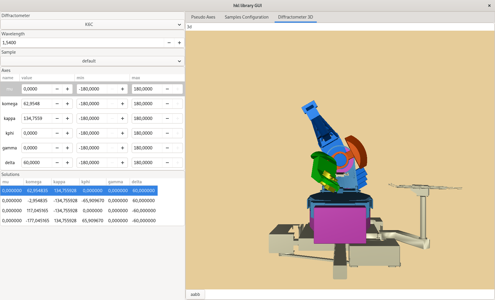
Figure 1: hkl library GUI interface

Features

mode computation (aka PseudoAxis).
item for different diffractometer geometries.
UB matrix computation:
- Busing & Levy with 2 reflections.
- simplex computation with more than 2 reflections using the GSL library.
- Eulerian angles to pre-orientate your sample.
Crystal lattice refinement:
- with more than 2 reflections, you can select which parameter must be fitted.
Pseudoaxes:
- psi, eulerians, q, …

Conventions

In this whole document, the next convention will be used to describe the diffractometers geometries:

right handed convention for all the angles.
direct space orthogonal base.
description of the diffractometer geometries is done with all axes values set to zero.

Diffraction

The crystal

A periodic crystal is the association of a pattern and a lattice. The pattern is located at each points of the lattice node. Positions of those nodes are given by:

\[ R_{uvw}=u\cdot\vec{a}+v\cdot\vec{b}+w\cdot\vec{c} \]

\(\vec{a}\), \(\vec{b}\), \(\vec{c}\) are the former vectors of a base of the space. u, v, w are integers. The pattern contains atoms associated to each lattice node. The purpose of diffraction is to study the interaction of this crystal (pattern + lattice) with X-rays.

Figure 2: Crystal direct lattice.

This lattice is defined by \(\vec{a}\), \(\vec{b}\), \(\vec{c}\) vectors, and the angles \(\alpha\), \(\beta\), \(\gamma\). In general cases, this lattice is not orthonormal.

Nevertheless, to compute the interaction of this real space lattice and the X-rays, it is convenient to define another lattice called the reciprocal space lattice defined like this:

\begin{eqnarray*} \vec{a}^{\star} & = & \tau\frac{\vec{b}\wedge\vec{c}}{\vec{a}\cdot(\vec{b}\wedge\vec{c})}\\ \vec{b}^{\star} & = & \tau\frac{\vec{c}\wedge\vec{a}}{\vec{b}\cdot(\vec{c}\wedge\vec{a})}\\ \vec{c}^{\star} & = & \tau\frac{\vec{a}\wedge\vec{b}}{\vec{c}\cdot(\vec{a}\wedge\vec{b})} \end{eqnarray*}

\(\tau=2\pi\) or \(\tau=1\) depending on the conventions.

It is then possible to define theses orthogonal properties:

\begin{eqnarray*} \vec{a}^{\star}\cdot\vec{a}=\tau & \vec{b}^{\star}\cdot\vec{a}=0 & \vec{c}^{\star}\cdot\vec{a}=0\\ \vec{a}^{\star}\cdot\vec{b}=0 & \vec{b}^{\star}\cdot\vec{b}=\tau & \vec{c}^{\star}\cdot\vec{b}=0\\ \vec{a}^{\star}\cdot\vec{c}=0 & \vec{b}^{\star}\cdot\vec{c}=0 & \vec{c}^{\star}\cdot\vec{c}=\tau \end{eqnarray*}

This reciprocal space lattice allows to write in a simpler form the interaction between the crystal and the X-rays. We often only know about \(\vec{a}\), \(\vec{b}\), \(\vec{c}\) vectors and the angles \(\alpha\), \(\beta\), \(\gamma\). Using the previous reciprocal equations, we can compute the reciprocal lattice this way:

\begin{eqnarray*} a^{\star} & = & \frac{\sin\alpha}{aD}\\ b^{\star} & = & \frac{\sin\beta}{bD}\\ c^{\star} & = & \frac{\sin\gamma}{cD} \end{eqnarray*}

where

\[ D=\sqrt{1-\cos^{2}\alpha-\cos^{2}\beta-\cos^{2}\gamma+2\cos\alpha\cos\beta\cos\gamma} \]

To compute the angles between the reciprocal space vectors, it is once again possible to use the previous reciprocal equations to obtain the sines and cosines of the angles \(\alpha^\star\), \(\beta^\star\) and \(\gamma^\star\):

\begin{eqnarray*} cosα^{*}=\frac{\cos\beta\cos\gamma-\cos\alpha}{\sin\beta\sin\gamma} & \, & sinα^{*}=\frac{D}{\sin\beta\sin\gamma}
cosβ^{*}=\frac{\cos\gamma\cos\alpha-\cos\beta}{\sin\gamma\sin\alpha} & \, & sinβ^{*}=\frac{D}{\sin\gamma\sin\alpha}
cosγ^{*}=\frac{\cos\alpha\cos\beta-\cos\gamma}{\sin\alpha\sin\beta} & \, & sinγ^{*}=\frac{D}{\sin\alpha\sin\beta} \end{eqnarray*}.

The volume of the lattice can be computed this way:

\[ V = abcD \]

\[ V = \vec{a} \dot (\vec{b} \wedge \vec{c}) = \vec{b} \dot (\vec{c} \wedge \vec{a}) = \vec{c} \dot (\vec{a} \wedge \vec{b}) \]

Diffraction

Let the incoming X-ray beam whose wave vector is \(\vec{k_{i}}\), \(|k_{i}|=\tau/\lambda\) where \(\lambda\) is the wavelength of the signal. And \(\vec{k_{d}}\) vector wavelength of the diffracted beam. There is diffraction if the diffraction vector \(\vec{q}\) can be expressed as follows:

\[ \vec{q}=\vec{k_{d}}-\vec{k_{i}}=h.\vec{a}^{*}+k.\vec{b}^{*}+l.\vec{c}^{*} \]

where \((h,k,l)\in\mathbb{N}^{3}\) and \((h,k,l)\neq(0,0,0)\). Theses indices \((h,k,l)\) are named Miller indices.

Another way of looking at things has been given by Bragg and that famous relationship:

\[ n\lambda=2d\sin\theta \]

where \(d\) is the inter-plan distance and \(n \in \mathbb{N}\).

The diffraction occurs for a unique \(\theta\) angle. Then we got \(\vec{q}\) perpendicular to the diffraction plans.

The Ewald construction allows to represent this diffraction condition in the reciprocal space.

Quaternions

Properties

The quaternions will be used to describe the diffractometer geometries. Theses quaternions can represent 3D rotations. There are different ways to describe such as complex numbers:

\[ q=a+bi+cj+dk \]

or

\[ q=[a,\vec{v}] \]

To compute the quaternion's norm, we can proceed like for complex numbers:

\[ \|q\|=\sqrt{a²+b²+c²+d²} \]

Its conjugate is:

\[ q^{*}=[a,-\vec{u}]=a-bi-cj-dk \]
Operations

The difference with complex number algebra is about non-commutativity.

\[ qp \neq pq \]
\begin{bmatrix} ~ & 1 & i & j & k \cr 1 & 1 & i & j & k \cr i & i & -1 & k & -j \cr j & j & -k & -1 & i \cr k & k & j & -i & -1 \end{bmatrix}
The product of two quaternions can be express by the Grassman product. So for two quaternions \(p\) and \(q\):
\begin{align*} q &= a+\vec{u} = a+bi+cj+dk\\ p &= t+\vec{v} = t+xi+yj+zk \end{align*}
we got:

\[ pq = at - \vec{u} \cdot \vec{v} + a \vec{v} + t \vec{u} + \vec{v} \times \vec{u} \]

or equivalent:

\[ pq = (at - bx - cy - dz) + (bt + ax + cz - dy) i + (ct + ay + dx - bz) j + (dt + az + by - cx) k \]
3D rotations

L'ensemble des quaternions unitaires (leur norme est égale à 1) est le groupe qui représente les rotations dans l'espace 3D. Si on a un vecteur unitaire \(\vec{u}\) et un angle de rotation \(\theta\) alors le quaternion \([\cos\frac{\theta}{2},\sin\frac{\theta}{2}\vec{u]}\) représente la rotation de \(\theta\) autour de l'axe \(\vec{u}\) dans le sens trigonométrique. Nous allons donc utiliser ces quaternions unitaires pour représenter les mouvements du diffractomètre.

Alors que dans le plan 2D une simple multiplication entre un nombre complex et le nombre \(e^{i\theta}\) permet de calculer simplement la rotation d'angle \(\theta\) autour de l'origine, dans l'espace 3D l'expression équivalente est:

\[ z'=qzq^{-1} \]

où \(q\) est le quaternion de norme 1 représentant la rotation dans l'espace et \(z\) le quaternion représentant le vecteur qui subit la rotation (sa partie réelle est nulle).

Dans le cas des quaternions de norme 1, il est très facile de calculer \(q^{-1}\). En effet l'inverse d'une rotation d'angle \(\theta\) est la rotation d'angle \(-\theta\). On a donc directement:

\[ q^{-1}=[\cos\frac{-\theta}{2},\sin\frac{-\theta}{2}\vec{u}]=[\cos\frac{\theta}{2},-\sin\frac{\theta}{2}\vec{u}]=q^{*} \]

Le passage aux matrices de rotation se fait par la formule suivante \(q\rightarrow M\).
\begin{bmatrix} a{{}^2}+b{{}^2}-c{{}^2}-d{{}^2} & 2bc-2ad & 2ac+2bd\\ 2ad+2bc & a{{}^2}-b{{}^2}+c{{}^2}-d{{}^2} & 2cd-2ab\\ 2bd-2ac & 2ab+2cd & a{{}^2}-b{{}^2}-c{{}^2}+d{{}^2} \end{bmatrix}
La composition de rotation se fait simplement en multipliant les quaternions entre eux. Si l'on a \(q\).

Modes de fonctionnement

To come.

Equations fondamentales

Le problème que nous devons résoudre est de calculer, pour une famille de plan \((h,k,l)\) donné, les angles de rotation du diffractomètre qui permettent de le mettre en condition de diffraction. Il faut donc exprimer les relations mathématiques qui lient les différents angles entre eux lorsque la condition de Bragg est vérifiée. L'équation fondamentale est la suivante:

\begin{align*} \left(\prod_{i}S_{i}\right)\cdot U\cdot B\cdot\vec{h} & =\left(\prod_{j}D_{j}-I\right)\cdot\vec{k_{i}}\\ R\cdot U\cdot B\cdot\vec{h} & =\vec{Q} \end{align*}

où \(\vec{h}\) est le vecteur \((h,k,l)\), \(\vec{k_{i}}\) est le vecteur incident, \(S_{i}\) les matrices de rotations des mouvements liés à l'échantillon, \(D_{j}\) les matrices de rotation des mouvements liés au détecteur, \(I\) la matrice identité, \(U\) la matrice d'orientation du cristal par rapport au repère de l'axe sur lequel ce dernier est monté et \(B\) la matrice de passage d'un repère non orthonormé (celui du cristal réciproque) à un repère orthonormé.

Calcule de B

Si l'on connaît les paramètres cristallins du cristal étudié, il est très simple de calculer \(B\):

\[ B = \]

\begin{bmatrix} a^{\star} & b^{\star}\cos\gamma^{\star} & c^{\star}\cos\beta^{\star}\\ 0 & b^{\star}\sin\gamma^{\star} & -c^{\star}\sin\beta^{\star}\cos\alpha\\ 0 & 0 & 1/c \end{bmatrix}

Calcule de U

Il existe plusieurs façons de calculer \(U\). Busing et Levy en ont proposé plusieurs. Nous allons présenter celle qui nécessite la mesure de seulement deux réflections ainsi que la connaissance des paramètres cristallins. Cette façon de calculer la matrice d'orientation \(U\) peut être généralisée à n'importe quel diffractomètre pour peu que la description des axes de rotation permette d'obtenir la matrice de rotation de la machine \(R\) et le vecteur de diffusion \(\vec{Q}\).

Il est également possible de calculer \(U\) sans la connaîssance des paramètres cristallins. Il faut alors faire un affinement des paramètres. Cela revient à minimiser une fonction. Nous allons utiliser la méthode du simplex pour trouver ce minimum et donc ajuster l'ensemble des paramètres cristallins ainsi que la matrice d'orientation.

Algorithme de Busing et Levy

L'idée est de se placer dans le repère de l'axe sur lequel est monté l'échantillon. On mesure deux réflections \((\vec{h}_{1},\vec{h}_{2})\) ainsi que leurs angles associés. Cela nous permet de calculer \(R\) et \(\vec{Q}\) pour chacune de ces reflections. Nous avons alors ce système:

\begin{eqnarray*} U\cdot B\cdot\vec{h}_{1} & = & \tilde{R}_{1}\cdot\vec{Q}_{1}\\ U\cdot B\cdot\vec{h}_{2} & = & \tilde{R}_{2}\cdot\vec{Q}_{2} \end{eqnarray*}

De façon à calculer facilement \(U\), il est intéressant de définir deux trièdres orthonormés \(T_{\vec{h}}\) et \(T_{\vec{Q}}\) à partir des vecteurs \((B\vec{h}_{1},B\vec{h}_{2})\) et \((\tilde{R}_{1}\vec{Q}_{1},\tilde{R}_{2}\vec{Q}_{2})\). On a alors très simplement:

\[ U \cdot T_{\vec{h}} = T_{\vec{Q}} \]

Et donc:

\[ U = T_{\vec{Q}} \cdot \tilde{T}_{\vec{h}} \]

Affinement par la méthode du simplex

Dans ce cas, nous ne connaissons pas la matrice \(B\), il faut donc mesurer plus que deux réflections pour ajuster les neuf paramètres. Six paramètres pour le crystal et trois pour la matrice d'orientation \(U\). Les trois paramètres qui permettent de représenter \(U\) sont en fait les angles d'Euler. Il faut donc être en mesure de passer d'une représentation eulérienne à cette matrice \(U\) et réciproquement.

\[ U = X \cdot Y \cdot Z \]

où \(X\) est la matrice de rotation suivant l'axe Ox et le premier angle d'Euler, \(Y\) la matrice de rotation suivant l'axe Oy et le deuxième angle d'Euler et \(Z\) la matrice du troisième angle d'Euler pour l'axe Oz.

\(X\)	\(Y\)	\(Z\)
\(\begin{bmatrix} 1 & 0 & 0\\ 0 & A & -B\\ 0 & B & A \end{bmatrix}\)	\(\begin{bmatrix}C & 0 & D\\0 & 1 & 0\\-D & 0 & C\end{bmatrix}\)	\(\begin{bmatrix}E & -F & 0\\F & E & 0\\0 & 0 & 1\end{bmatrix}\)

et donc:

\[ U= \]

\begin{bmatrix} CE & -CF & D\\ BDE+AF & -BDF+AE & -BC\\ -ADE+BF & ADF+BE & AC \end{bmatrix}

Il est donc facile de passer des angles d'Euler à la matrice d'orientation.

Il faut maintenant faire la transformation inverse de la matrice \(U\) vers les angles d'Euler.

2. PseudoAxes

This section describes the calculations done by the library for the different kind of pseudo-axes.

General process

First Solution

The hkl library uses the gsl library in order to find the first valid solution.

Multiplication of the solutions

Once we have got the first solution, different strategies are applied in order to generate more solutions.

Geometry Multiplication

For kappa diffractometers, once you have one solution, it is possible to generate another one using a property of this geometry. (Left arm and right arm).

Restrains of the Solutions

We apply then some constrains to reduce these solutions to only a bunch of acceptable ones. Usually we take the axis range into account.

Eulerians to Kappa angles

1st solution:

\begin{eqnarray*} \kappa_\omega & = & \omega - p + \frac{\pi}{2} \\ \kappa & = & 2 \arcsin\left(\frac{\sin\frac{\chi}{2}}{\sin\alpha}\right) \\ \kappa_\phi & = & \phi - p - \frac{\pi}{2} \end{eqnarray*}

or 2nd one:

\begin{eqnarray*} \kappa_\omega & = & \omega - p - \frac{\pi}{2} \\ \kappa & = & -2 \arcsin\left(\frac{\sin\frac{\chi}{2}}{\sin\alpha}\right) \\ \kappa_\phi & = & \phi - p + \frac{\pi}{2} \end{eqnarray*}

where

\[ p = \arcsin\left(\frac{\tan\frac{\chi}{2}}{\tan\alpha}\right) \]

and \(\alpha\) is the angle of the kappa axis with the \(\vec{y}\) axis.

Kappa to Eulerian angles

1st solution:

\begin{eqnarray*} \omega & = & \kappa_\omega + p - \frac{\pi}{2} \\ \chi & = & 2 \arcsin\left(\sin\frac{\kappa}{2} \sin\alpha\right) \\ \phi & = & \kappa_\phi + p + \frac{\pi}{2} \end{eqnarray*}

or 2nd one:

\begin{eqnarray*} \omega & = & \kappa_\omega + p + \frac{\pi}{2} \\ \chi & = & -2 \arcsin\left(\sin\frac{\kappa}{2} \sin\alpha\right) \\ \phi & = & \kappa_\phi + p - \frac{\pi}{2} \end{eqnarray*}

where

\[ p = \arctan\left(\tan\frac{\kappa}{2} \cos\alpha\right) \]

Figure 3: \(\omega = 0\), \(\chi = 0\), \(\phi = 0\), 1st solution

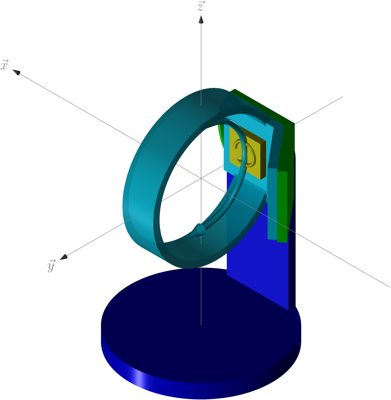
Figure 4: \(\omega = 0\), \(\chi = 0\), \(\phi = 0\), 2nd solution

Figure 5: \(\omega = 0\), \(\chi = 90\), \(\phi = 0\), 1st solution

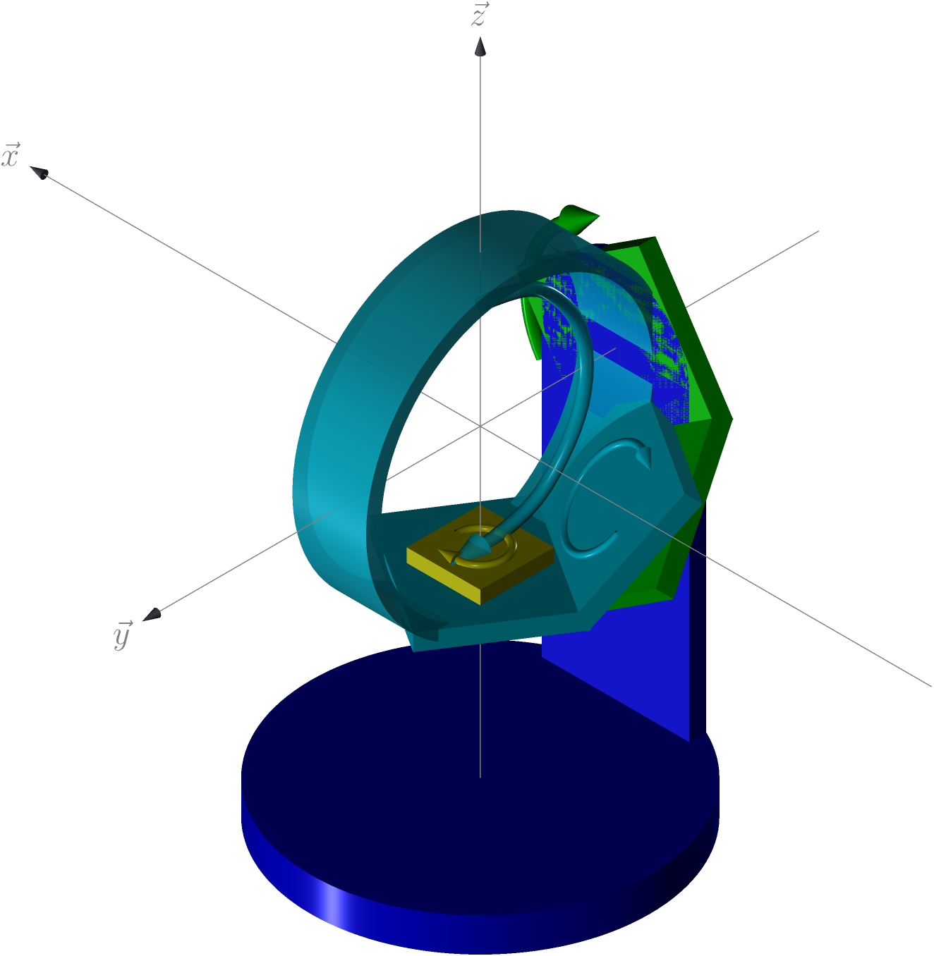
Figure 6: \(\omega = 0\), \(\chi = 90\), \(\phi = 0\), 2nd solution

Qper and Qpar

This pseudo axis engine computes the perpendicular (\(\left|\left|\vec{Q_\text{per}}\right|\right|\)) and parallel (\(\left|\left|\vec{Q_\text{par}}\right|\right|\)) contribution of \(\vec{Q}\) relatively to the surface of the sample defined by the \(\vec{n}\) vector.

\begin{eqnarray*} \vec{q} & = & \vec{k_\text{f}} - \vec{k_\text{i}} \\ \vec{q} & = & \vec{q_\text{per}} + \vec{q_\text{par}} \\ \vec{q_\text{per}} & = & \frac{\vec{q} \cdot \vec{n}}{\left|\left|\vec{n}\right|\right|} \frac{\vec{n}}{\left|\left|\vec{n}\right|\right|} \end{eqnarray*}

3. Diffractometers

Warning

This section is automatically generating by introspecting the hkl library.

APS POLAR

Axes:

"tau": rotation around the [0.0, -1.0, 0.0] axis
"mu": rotation around the [0.0, 0.0, 1.0] axis
"chi": rotation around the [1.0, 0.0, 0.0] axis
"phi": rotation around the [0.0, 0.0, 1.0] axis
"gamma": rotation around the [0.0, 0.0, 1.0] axis
"delta": rotation around the [0.0, -1.0, 0.0] axis

Engines:

"hkl":
- pseudo axes:
  - "h" : h coordinate of the diffracting plan
  - "k" : k coordinate of the diffracting plan
  - "l" : l coordinate of the diffracting plan
- mode: "4-circles constant phi horizontal"
  - axes (read) : "tau", "mu", "chi", "phi", "gamma", "delta"
  - axes (write): "mu", "chi", "gamma"
  - parameters: No parameter
- mode: "zaxis + alpha-fixed"
  - axes (read) : "tau", "mu", "chi", "phi", "gamma", "delta"
  - axes (write): "mu", "gamma", "delta"
  - parameters: No parameter
- mode: "zaxis + beta-fixed"
  - axes (read) : "tau", "mu", "chi", "phi", "gamma", "delta"
  - axes (write): "tau", "gamma", "delta"
  - parameters: No parameter
- mode: "zaxis + alpha=beta"
  - axes (read) : "tau", "mu", "chi", "phi", "gamma", "delta"
  - axes (write): "tau", "mu", "gamma", "delta"
  - parameters: No parameter
- mode: "4-circles bissecting horizontal"
  - axes (read) : "tau", "mu", "chi", "phi", "gamma", "delta"
  - axes (write): "mu", "chi", "phi", "gamma"
  - parameters: No parameter
- mode: "4-circles constant mu horizontal"
  - axes (read) : "tau", "mu", "chi", "phi", "gamma", "delta"
  - axes (write): "chi", "phi", "gamma"
  - parameters: No parameter
- mode: "4-circles constant chi horizontal"
  - axes (read) : "tau", "mu", "chi", "phi", "gamma", "delta"
  - axes (write): "mu", "phi", "gamma"
  - parameters: No parameter
- mode: "lifting detector tau"
  - axes (read) : "tau", "mu", "chi", "phi", "gamma", "delta"
  - axes (write): "tau", "gamma", "delta"
  - parameters: No parameter
- mode: "lifting detector mu"
  - axes (read) : "tau", "mu", "chi", "phi", "gamma", "delta"
  - axes (write): "mu", "gamma", "delta"
  - parameters: No parameter
- mode: "lifting detector chi"
  - axes (read) : "tau", "mu", "chi", "phi", "gamma", "delta"
  - axes (write): "chi", "gamma", "delta"
  - parameters: No parameter
- mode: "lifting detector phi"
  - axes (read) : "tau", "mu", "chi", "phi", "gamma", "delta"
  - axes (write): "phi", "gamma", "delta"
  - parameters: No parameter
- mode: "psi constant horizontal"
  - axes (read) : "tau", "mu", "chi", "phi", "gamma", "delta"
  - axes (write): "mu", "chi", "phi", "gamma"
  - parameters:
    - h2 [1.0]: h coordinate of the reference plan
    - k2 [0.0]: k coordinate of the reference plan
    - l2 [0.0]: l coordinate of the reference plan
    - psi [0.0]: expected angle between the reference and the diffraction plans
- mode: "psi constant vertical"
  - axes (read) : "tau", "mu", "chi", "phi", "gamma", "delta"
  - axes (write): "tau", "chi", "phi", "delta"
  - parameters:
    - h2 [1.0]: h coordinate of the reference plan
    - k2 [0.0]: k coordinate of the reference plan
    - l2 [0.0]: l coordinate of the reference plan
    - psi [0.0]: expected angle between the reference and the diffraction plans
"psi":
- pseudo axes:
  - "psi" : angle between the reference vector and the diffraction plan
- mode: "psi_vertical"
  - axes (read) : "tau", "mu", "chi", "phi", "gamma", "delta"
  - axes (write): "mu", "chi", "phi", "delta"
  - parameters:
    - h2 [1.0]: h coordinate of the reference plan
    - k2 [1.0]: k coordinate of the reference plan
    - l2 [1.0]: l coordinate of the reference plan

E4CH

Axes:

"omega": rotation around the [0.0, 0.0, 1.0] axis
"chi": rotation around the [1.0, 0.0, 0.0] axis
"phi": rotation around the [0.0, 0.0, 1.0] axis
"tth": rotation around the [0.0, 0.0, 1.0] axis

Engines:

"hkl":
- pseudo axes:
  - "h" : h coordinate of the diffracting plan
  - "k" : k coordinate of the diffracting plan
  - "l" : l coordinate of the diffracting plan
- mode: "bissector"
  - axes (read) : "omega", "chi", "phi", "tth"
  - axes (write): "omega", "chi", "phi", "tth"
  - parameters: No parameter
- mode: "constant_omega"
  - axes (read) : "omega", "chi", "phi", "tth"
  - axes (write): "chi", "phi", "tth"
  - parameters: No parameter
- mode: "constant_chi"
  - axes (read) : "omega", "chi", "phi", "tth"
  - axes (write): "omega", "phi", "tth"
  - parameters: No parameter
- mode: "constant_phi"
  - axes (read) : "omega", "chi", "phi", "tth"
  - axes (write): "omega", "chi", "tth"
  - parameters: No parameter
- mode: "double_diffraction"
  - axes (read) : "omega", "chi", "phi", "tth"
  - axes (write): "omega", "chi", "phi", "tth"
  - parameters:
    - h2 [1.0]: h coordinate of the second diffracting plan
    - k2 [1.0]: k coordinate of the second diffracting plan
    - l2 [1.0]: l coordinate of the second diffracting plan
- mode: "psi_constant"
  - axes (read) : "omega", "chi", "phi", "tth"
  - axes (write): "omega", "chi", "phi", "tth"
  - parameters:
    - h2 [1.0]: h coordinate of the reference plan
    - k2 [1.0]: k coordinate of the reference plan
    - l2 [1.0]: l coordinate of the reference plan
    - psi [0.0]: expected angle between the reference and the diffraction plans
"psi":
- pseudo axes:
  - "psi" : angle between the reference vector and the diffraction plan
- mode: "psi"
  - axes (read) : "omega", "chi", "phi", "tth"
  - axes (write): "omega", "chi", "phi", "tth"
  - parameters:
    - h2 [1.0]: h coordinate of the reference plan
    - k2 [1.0]: k coordinate of the reference plan
    - l2 [1.0]: l coordinate of the reference plan
"q":
- pseudo axes:
  - "q" : the norm of \(\vec{q}\)
- mode: "q"
  - axes (read) : "tth"
  - axes (write): "tth"
  - parameters: No parameter
"incidence":
- pseudo axes:
  - "incidence" : incidence of the incomming beam.
  - "azimuth" : azimuth of the sample surface (projection of \(\vec{n}\) on the \(yOz\) plan
- mode: "incidence"
  - axes (read) : "omega", "chi", "phi"
  - axes (write):
  - parameters:
    - x [0.0]: the x coordinate of the surface \(\vec{n}\)
    - y [1.0]: the y coordinate of the surface \(\vec{n}\)
    - z [0.0]: the z coordinate of the surface \(\vec{n}\)
"emergence":
- pseudo axes:
  - "emergence" : incidence of the outgoing beam.
  - "azimuth" : azimuth of the sample surface (projection of \(\vec{n}\) on the \(yOz\) plan
- mode: "emergence"
  - axes (read) : "omega", "chi", "phi", "tth"
  - axes (write):
  - parameters:
    - x [0.0]: the x coordinate of the surface \(\vec{n}\)
    - y [1.0]: the y coordinate of the surface \(\vec{n}\)
    - z [0.0]: the z coordinate of the surface \(\vec{n}\)

E4CV

Axes:

"omega": rotation around the [0.0, -1.0, 0.0] axis
"chi": rotation around the [1.0, 0.0, 0.0] axis
"phi": rotation around the [0.0, -1.0, 0.0] axis
"tth": rotation around the [0.0, -1.0, 0.0] axis

Engines:

"hkl":
- pseudo axes:
  - "h" : h coordinate of the diffracting plan
  - "k" : k coordinate of the diffracting plan
  - "l" : l coordinate of the diffracting plan
- mode: "bissector"
  - axes (read) : "omega", "chi", "phi", "tth"
  - axes (write): "omega", "chi", "phi", "tth"
  - parameters: No parameter
- mode: "constant_omega"
  - axes (read) : "omega", "chi", "phi", "tth"
  - axes (write): "chi", "phi", "tth"
  - parameters: No parameter
- mode: "constant_chi"
  - axes (read) : "omega", "chi", "phi", "tth"
  - axes (write): "omega", "phi", "tth"
  - parameters: No parameter
- mode: "constant_phi"
  - axes (read) : "omega", "chi", "phi", "tth"
  - axes (write): "omega", "chi", "tth"
  - parameters: No parameter
- mode: "double_diffraction"
  - axes (read) : "omega", "chi", "phi", "tth"
  - axes (write): "omega", "chi", "phi", "tth"
  - parameters:
    - h2 [1.0]: h coordinate of the second diffracting plan
    - k2 [1.0]: k coordinate of the second diffracting plan
    - l2 [1.0]: l coordinate of the second diffracting plan
- mode: "psi_constant"
  - axes (read) : "omega", "chi", "phi", "tth"
  - axes (write): "omega", "chi", "phi", "tth"
  - parameters:
    - h2 [1.0]: h coordinate of the reference plan
    - k2 [1.0]: k coordinate of the reference plan
    - l2 [1.0]: l coordinate of the reference plan
    - psi [0.0]: expected angle between the reference and the diffraction plans
"psi":
- pseudo axes:
  - "psi" : angle between the reference vector and the diffraction plan
- mode: "psi"
  - axes (read) : "omega", "chi", "phi", "tth"
  - axes (write): "omega", "chi", "phi", "tth"
  - parameters:
    - h2 [1.0]: h coordinate of the reference plan
    - k2 [1.0]: k coordinate of the reference plan
    - l2 [1.0]: l coordinate of the reference plan
"q":
- pseudo axes:
  - "q" : the norm of \(\vec{q}\)
- mode: "q"
  - axes (read) : "tth"
  - axes (write): "tth"
  - parameters: No parameter
"incidence":
- pseudo axes:
  - "incidence" : incidence of the incomming beam.
  - "azimuth" : azimuth of the sample surface (projection of \(\vec{n}\) on the \(yOz\) plan
- mode: "incidence"
  - axes (read) : "omega", "chi", "phi"
  - axes (write):
  - parameters:
    - x [0.0]: the x coordinate of the surface \(\vec{n}\)
    - y [1.0]: the y coordinate of the surface \(\vec{n}\)
    - z [0.0]: the z coordinate of the surface \(\vec{n}\)
"emergence":
- pseudo axes:
  - "emergence" : incidence of the outgoing beam.
  - "azimuth" : azimuth of the sample surface (projection of \(\vec{n}\) on the \(yOz\) plan
- mode: "emergence"
  - axes (read) : "omega", "chi", "phi", "tth"
  - axes (write):
  - parameters:
    - x [0.0]: the x coordinate of the surface \(\vec{n}\)
    - y [1.0]: the y coordinate of the surface \(\vec{n}\)
    - z [0.0]: the z coordinate of the surface \(\vec{n}\)

E6C

Axes:

"mu": rotation around the [0.0, 0.0, 1.0] axis
"omega": rotation around the [0.0, -1.0, 0.0] axis
"chi": rotation around the [1.0, 0.0, 0.0] axis
"phi": rotation around the [0.0, -1.0, 0.0] axis
"gamma": rotation around the [0.0, 0.0, 1.0] axis
"delta": rotation around the [0.0, -1.0, 0.0] axis

Engines:

"hkl":
- pseudo axes:
  - "h" : h coordinate of the diffracting plan
  - "k" : k coordinate of the diffracting plan
  - "l" : l coordinate of the diffracting plan
- mode: "bissector_vertical"
  - axes (read) : "mu", "omega", "chi", "phi", "gamma", "delta"
  - axes (write): "omega", "chi", "phi", "delta"
  - parameters: No parameter
- mode: "constant_omega_vertical"
  - axes (read) : "mu", "omega", "chi", "phi", "gamma", "delta"
  - axes (write): "chi", "phi", "delta"
  - parameters: No parameter
- mode: "constant_chi_vertical"
  - axes (read) : "mu", "omega", "chi", "phi", "gamma", "delta"
  - axes (write): "omega", "phi", "delta"
  - parameters: No parameter
- mode: "constant_phi_vertical"
  - axes (read) : "mu", "omega", "chi", "phi", "gamma", "delta"
  - axes (write): "omega", "chi", "delta"
  - parameters: No parameter
- mode: "lifting_detector_phi"
  - axes (read) : "mu", "omega", "chi", "phi", "gamma", "delta"
  - axes (write): "phi", "gamma", "delta"
  - parameters: No parameter
- mode: "lifting_detector_omega"
  - axes (read) : "mu", "omega", "chi", "phi", "gamma", "delta"
  - axes (write): "omega", "gamma", "delta"
  - parameters: No parameter
- mode: "lifting_detector_mu"
  - axes (read) : "mu", "omega", "chi", "phi", "gamma", "delta"
  - axes (write): "mu", "gamma", "delta"
  - parameters: No parameter
- mode: "double_diffraction_vertical"
  - axes (read) : "mu", "omega", "chi", "phi", "gamma", "delta"
  - axes (write): "omega", "chi", "phi", "delta"
  - parameters:
    - h2 [1.0]: h coordinate of the second diffracting plan
    - k2 [1.0]: k coordinate of the second diffracting plan
    - l2 [1.0]: l coordinate of the second diffracting plan
- mode: "bissector_horizontal"
  - axes (read) : "mu", "omega", "chi", "phi", "gamma", "delta"
  - axes (write): "mu", "omega", "chi", "phi", "gamma"
  - parameters: No parameter
- mode: "double_diffraction_horizontal"
  - axes (read) : "mu", "omega", "chi", "phi", "gamma", "delta"
  - axes (write): "mu", "chi", "phi", "gamma"
  - parameters:
    - h2 [1.0]: h coordinate of the second diffracting plan
    - k2 [1.0]: k coordinate of the second diffracting plan
    - l2 [1.0]: l coordinate of the second diffracting plan
- mode: "psi_constant_vertical"
  - axes (read) : "mu", "omega", "chi", "phi", "gamma", "delta"
  - axes (write): "omega", "chi", "phi", "delta"
  - parameters:
    - h2 [1.0]: h coordinate of the reference plan
    - k2 [0.0]: k coordinate of the reference plan
    - l2 [0.0]: l coordinate of the reference plan
    - psi [0.0]: expected angle between the reference and the diffraction plans
- mode: "psi_constant_horizontal"
  - axes (read) : "mu", "omega", "chi", "phi", "gamma", "delta"
  - axes (write): "omega", "chi", "phi", "gamma"
  - parameters:
    - h2 [1.0]: h coordinate of the reference plan
    - k2 [1.0]: k coordinate of the reference plan
    - l2 [1.0]: l coordinate of the reference plan
    - psi [0.0]: expected angle between the reference and the diffraction plans
- mode: "constant_mu_horizontal"
  - axes (read) : "mu", "omega", "chi", "phi", "gamma", "delta"
  - axes (write): "chi", "phi", "gamma"
  - parameters: No parameter
"psi":
- pseudo axes:
  - "psi" : angle between the reference vector and the diffraction plan
- mode: "psi_vertical"
  - axes (read) : "mu", "omega", "chi", "phi", "gamma", "delta"
  - axes (write): "omega", "chi", "phi", "delta"
  - parameters:
    - h2 [1.0]: h coordinate of the reference plan
    - k2 [1.0]: k coordinate of the reference plan
    - l2 [1.0]: l coordinate of the reference plan
"q2":
- pseudo axes:
  - "q" : the norm of \(\vec{q}\)
  - "alpha" : angle of the projection of \(\vec{q}\) on the \(yOz\) plan and \(\vec{y}\)
- mode: "q2"
  - axes (read) : "gamma", "delta"
  - axes (write): "gamma", "delta"
  - parameters: No parameter
"qper_qpar":
- pseudo axes:
  - "qper" : perpendicular component of \(\vec{q}\) along the normal of the sample surface
  - "qpar" : parallel component of \(\vec{q}\)
- mode: "qper_qpar"
  - axes (read) : "gamma", "delta"
  - axes (write): "gamma", "delta"
  - parameters:
    - x [0.0]: the x coordinate of the surface \(\vec{n}\)
    - y [1.0]: the y coordinate of the surface \(\vec{n}\)
    - z [0.0]: the z coordinate of the surface \(\vec{n}\)
"tth2":
- pseudo axes:
  - "tth" : the \(2 \theta\) angle
  - "alpha" : angle of the projection of \(\vec{q}\) on the \(yOz\) plan and \(\vec{y}\)
- mode: "tth2"
  - axes (read) : "gamma", "delta"
  - axes (write): "gamma", "delta"
  - parameters: No parameter
"incidence":
- pseudo axes:
  - "incidence" : incidence of the incomming beam.
  - "azimuth" : azimuth of the sample surface (projection of \(\vec{n}\) on the \(yOz\) plan
- mode: "incidence"
  - axes (read) : "mu", "omega", "chi", "phi"
  - axes (write):
  - parameters:
    - x [0.0]: the x coordinate of the surface \(\vec{n}\)
    - y [1.0]: the y coordinate of the surface \(\vec{n}\)
    - z [0.0]: the z coordinate of the surface \(\vec{n}\)
"emergence":
- pseudo axes:
  - "emergence" : incidence of the outgoing beam.
  - "azimuth" : azimuth of the sample surface (projection of \(\vec{n}\) on the \(yOz\) plan
- mode: "emergence"
  - axes (read) : "mu", "omega", "chi", "phi", "gamma", "delta"
  - axes (write):
  - parameters:
    - x [0.0]: the x coordinate of the surface \(\vec{n}\)
    - y [1.0]: the y coordinate of the surface \(\vec{n}\)
    - z [0.0]: the z coordinate of the surface \(\vec{n}\)

ESRF BM28 PSIC

Axes:

"mu": rotation around the [0.0, 0.0, 1.0] axis
"eta": rotation around the [0.0, -1.0, 0.0] axis
"chi": rotation around the [1.0, 0.0, 0.0] axis
"phi": rotation around the [0.0, -1.0, 0.0] axis
"nu": rotation around the [0.0, 0.0, 1.0] axis
"delta": rotation around the [0.0, -1.0, 0.0] axis

Engines:

"hkl":
- pseudo axes:
  - "h" : h coordinate of the diffracting plan
  - "k" : k coordinate of the diffracting plan
  - "l" : l coordinate of the diffracting plan
- mode: "constant_nu_coplanar"
  - axes (read) : "mu", "eta", "chi", "phi", "nu", "delta"
  - axes (write): "eta", "phi", "delta"
  - parameters: No parameter
- mode: "constant_delta_coplanar"
  - axes (read) : "mu", "eta", "chi", "phi", "nu", "delta"
  - axes (write): "eta", "phi", "nu"
  - parameters: No parameter
- mode: "constant_eta_noncoplanar"
  - axes (read) : "mu", "eta", "chi", "phi", "nu", "delta"
  - axes (write): "phi", "nu", "delta"
  - parameters: No parameter
"incidence":
- pseudo axes:
  - "incidence" : incidence of the incomming beam.
  - "azimuth" : azimuth of the sample surface (projection of \(\vec{n}\) on the \(yOz\) plan
- mode: "incidence"
  - axes (read) : "mu", "eta", "chi", "phi"
  - axes (write):
  - parameters:
    - x [0.0]: the x coordinate of the surface \(\vec{n}\)
    - y [1.0]: the y coordinate of the surface \(\vec{n}\)
    - z [0.0]: the z coordinate of the surface \(\vec{n}\)
"emergence":
- pseudo axes:
  - "emergence" : incidence of the outgoing beam.
  - "azimuth" : azimuth of the sample surface (projection of \(\vec{n}\) on the \(yOz\) plan
- mode: "emergence"
  - axes (read) : "mu", "eta", "chi", "phi", "nu", "delta"
  - axes (write):
  - parameters:
    - x [0.0]: the x coordinate of the surface \(\vec{n}\)
    - y [1.0]: the y coordinate of the surface \(\vec{n}\)
    - z [0.0]: the z coordinate of the surface \(\vec{n}\)

ESRF ID01 PSIC

Axes:

"mu": rotation around the [0.0, 0.0, -1.0] axis
"eta": rotation around the [0.0, -1.0, 0.0] axis
"phi": rotation around the [0.0, 0.0, -1.0] axis
"nu": rotation around the [0.0, 0.0, -1.0] axis
"delta": rotation around the [0.0, -1.0, 0.0] axis

Engines:

"hkl":
- pseudo axes:
  - "h" : h coordinate of the diffracting plan
  - "k" : k coordinate of the diffracting plan
  - "l" : l coordinate of the diffracting plan
- mode: "constant_nu_coplanar"
  - axes (read) : "mu", "eta", "phi", "nu", "delta"
  - axes (write): "eta", "phi", "delta"
  - parameters: No parameter
- mode: "constant_delta_coplanar"
  - axes (read) : "mu", "eta", "phi", "nu", "delta"
  - axes (write): "eta", "phi", "nu"
  - parameters: No parameter
- mode: "constant_eta_noncoplanar"
  - axes (read) : "mu", "eta", "phi", "nu", "delta"
  - axes (write): "phi", "nu", "delta"
  - parameters: No parameter

K4CV

Axes:

"komega": rotation around the [0.0, -1.0, 0.0] axis
"kappa": rotation around the [0.0, -0.6427876096865394, -0.766044443118978] axis
"kphi": rotation around the [0.0, -1.0, 0.0] axis
"tth": rotation around the [0.0, -1.0, 0.0] axis

Engines:

"hkl":
- pseudo axes:
  - "h" : h coordinate of the diffracting plan
  - "k" : k coordinate of the diffracting plan
  - "l" : l coordinate of the diffracting plan
- mode: "bissector"
  - axes (read) : "komega", "kappa", "kphi", "tth"
  - axes (write): "komega", "kappa", "kphi", "tth"
  - parameters: No parameter
- mode: "constant_omega"
  - axes (read) : "komega", "kappa", "kphi", "tth"
  - axes (write): "komega", "kappa", "kphi", "tth"
  - parameters:
    - omega [0.0]: the freezed value
- mode: "constant_chi"
  - axes (read) : "komega", "kappa", "kphi", "tth"
  - axes (write): "komega", "kappa", "kphi", "tth"
  - parameters:
    - chi [0.0]: the freezed value
- mode: "constant_phi"
  - axes (read) : "komega", "kappa", "kphi", "tth"
  - axes (write): "komega", "kappa", "kphi", "tth"
  - parameters:
    - phi [0.0]: the freezed value
- mode: "double_diffraction"
  - axes (read) : "komega", "kappa", "kphi", "tth"
  - axes (write): "komega", "kappa", "kphi", "tth"
  - parameters:
    - h2 [1.0]: h coordinate of the second diffracting plan
    - k2 [1.0]: k coordinate of the second diffracting plan
    - l2 [1.0]: l coordinate of the second diffracting plan
- mode: "psi_constant"
  - axes (read) : "komega", "kappa", "kphi", "tth"
  - axes (write): "komega", "kappa", "kphi", "tth"
  - parameters:
    - h2 [1.0]: h coordinate of the reference plan
    - k2 [1.0]: k coordinate of the reference plan
    - l2 [1.0]: l coordinate of the reference plan
    - psi [0.0]: expected angle between the reference and the diffraction plans
"eulerians":
- pseudo axes:
  - "omega" : omega equivalent for a four circle eulerian geometry
  - "chi" : chi equivalent for a four circle eulerian geometry
  - "phi" : phi equivalent for a four circle eulerian geometry
- mode: "eulerians"
  - axes (read) : "komega", "kappa", "kphi"
  - axes (write): "komega", "kappa", "kphi"
  - parameters:
    - solutions [1.0]: (0/1) to select the first or second solution
"psi":
- pseudo axes:
  - "psi" : angle between the reference vector and the diffraction plan
- mode: "psi"
  - axes (read) : "komega", "kappa", "kphi", "tth"
  - axes (write): "komega", "kappa", "kphi", "tth"
  - parameters:
    - h2 [1.0]: h coordinate of the reference plan
    - k2 [1.0]: k coordinate of the reference plan
    - l2 [1.0]: l coordinate of the reference plan
"q":
- pseudo axes:
  - "q" : the norm of \(\vec{q}\)
- mode: "q"
  - axes (read) : "tth"
  - axes (write): "tth"
  - parameters: No parameter
"incidence":
- pseudo axes:
  - "incidence" : incidence of the incomming beam.
  - "azimuth" : azimuth of the sample surface (projection of \(\vec{n}\) on the \(yOz\) plan
- mode: "incidence"
  - axes (read) : "komega", "kappa", "kphi"
  - axes (write):
  - parameters:
    - x [0.0]: the x coordinate of the surface \(\vec{n}\)
    - y [1.0]: the y coordinate of the surface \(\vec{n}\)
    - z [0.0]: the z coordinate of the surface \(\vec{n}\)
"emergence":
- pseudo axes:
  - "emergence" : incidence of the outgoing beam.
  - "azimuth" : azimuth of the sample surface (projection of \(\vec{n}\) on the \(yOz\) plan
- mode: "emergence"
  - axes (read) : "komega", "kappa", "kphi", "tth"
  - axes (write):
  - parameters:
    - x [0.0]: the x coordinate of the surface \(\vec{n}\)
    - y [1.0]: the y coordinate of the surface \(\vec{n}\)
    - z [0.0]: the z coordinate of the surface \(\vec{n}\)

K6C

Axes:

"mu": rotation around the [0.0, 0.0, 1.0] axis
"komega": rotation around the [0.0, -1.0, 0.0] axis
"kappa": rotation around the [0.0, -0.6427876096865394, -0.766044443118978] axis
"kphi": rotation around the [0.0, -1.0, 0.0] axis
"gamma": rotation around the [0.0, 0.0, 1.0] axis
"delta": rotation around the [0.0, -1.0, 0.0] axis

Engines:

"hkl":
- pseudo axes:
  - "h" : h coordinate of the diffracting plan
  - "k" : k coordinate of the diffracting plan
  - "l" : l coordinate of the diffracting plan
- mode: "bissector_vertical"
  - axes (read) : "mu", "komega", "kappa", "kphi", "gamma", "delta"
  - axes (write): "komega", "kappa", "kphi", "delta"
  - parameters: No parameter
- mode: "constant_omega_vertical"
  - axes (read) : "mu", "komega", "kappa", "kphi", "gamma", "delta"
  - axes (write): "komega", "kappa", "kphi", "delta"
  - parameters:
    - omega [0.0]: the freezed value
- mode: "constant_chi_vertical"
  - axes (read) : "mu", "komega", "kappa", "kphi", "gamma", "delta"
  - axes (write): "komega", "kappa", "kphi", "delta"
  - parameters:
    - chi [0.0]: the freezed value
- mode: "constant_phi_vertical"
  - axes (read) : "mu", "komega", "kappa", "kphi", "gamma", "delta"
  - axes (write): "komega", "kappa", "kphi", "delta"
  - parameters:
    - phi [0.0]: the freezed value
- mode: "lifting_detector_kphi"
  - axes (read) : "mu", "komega", "kappa", "kphi", "gamma", "delta"
  - axes (write): "kphi", "gamma", "delta"
  - parameters: No parameter
- mode: "lifting_detector_komega"
  - axes (read) : "mu", "komega", "kappa", "kphi", "gamma", "delta"
  - axes (write): "komega", "gamma", "delta"
  - parameters: No parameter
- mode: "lifting_detector_mu"
  - axes (read) : "mu", "komega", "kappa", "kphi", "gamma", "delta"
  - axes (write): "mu", "gamma", "delta"
  - parameters: No parameter
- mode: "double_diffraction_vertical"
  - axes (read) : "mu", "komega", "kappa", "kphi", "gamma", "delta"
  - axes (write): "komega", "kappa", "kphi", "delta"
  - parameters:
    - h2 [1.0]: h coordinate of the second diffracting plan
    - k2 [1.0]: k coordinate of the second diffracting plan
    - l2 [1.0]: l coordinate of the second diffracting plan
- mode: "bissector_horizontal"
  - axes (read) : "mu", "komega", "kappa", "kphi", "gamma", "delta"
  - axes (write): "mu", "komega", "kappa", "kphi", "gamma"
  - parameters: No parameter
- mode: "constant_phi_horizontal"
  - axes (read) : "mu", "komega", "kappa", "kphi", "gamma", "delta"
  - axes (write): "mu", "komega", "kappa", "kphi", "gamma"
  - parameters:
    - phi [0.0]: the freezed value
- mode: "constant_kphi_horizontal"
  - axes (read) : "mu", "komega", "kappa", "kphi", "gamma", "delta"
  - axes (write): "mu", "komega", "kappa", "gamma"
  - parameters: No parameter
- mode: "double_diffraction_horizontal"
  - axes (read) : "mu", "komega", "kappa", "kphi", "gamma", "delta"
  - axes (write): "mu", "komega", "kappa", "kphi", "gamma"
  - parameters:
    - h2 [1.0]: h coordinate of the second diffracting plan
    - k2 [1.0]: k coordinate of the second diffracting plan
    - l2 [1.0]: l coordinate of the second diffracting plan
- mode: "psi_constant_vertical"
  - axes (read) : "mu", "komega", "kappa", "kphi", "gamma", "delta"
  - axes (write): "komega", "kappa", "kphi", "delta"
  - parameters:
    - h2 [1.0]: h coordinate of the reference plan
    - k2 [1.0]: k coordinate of the reference plan
    - l2 [1.0]: l coordinate of the reference plan
    - psi [0.0]: expected angle between the reference and the diffraction plans
- mode: "constant_incidence"
  - axes (read) : "mu", "komega", "kappa", "kphi", "gamma", "delta"
  - axes (write): "komega", "kappa", "kphi", "gamma", "delta"
  - parameters:
    - x [1.0]: the x coordinate of the surface \(\vec{n}\)
    - y [1.0]: the y coordinate of the surface \(\vec{n}\)
    - z [1.0]: the z coordinate of the surface \(\vec{n}\)
    - incidence [0.0]: expected incidence of the incoming beam \(\vec{k_i}\) on the surface.
    - azimuth [90.0]: expected azimuth
"eulerians":
- pseudo axes:
  - "omega" : omega equivalent for a four circle eulerian geometry
  - "chi" : chi equivalent for a four circle eulerian geometry
  - "phi" : phi equivalent for a four circle eulerian geometry
- mode: "eulerians"
  - axes (read) : "komega", "kappa", "kphi"
  - axes (write): "komega", "kappa", "kphi"
  - parameters:
    - solutions [1.0]: (0/1) to select the first or second solution
"psi":
- pseudo axes:
  - "psi" : angle between the reference vector and the diffraction plan
- mode: "psi_vertical"
  - axes (read) : "mu", "komega", "kappa", "kphi", "gamma", "delta"
  - axes (write): "komega", "kappa", "kphi", "delta"
  - parameters:
    - h2 [1.0]: h coordinate of the reference plan
    - k2 [1.0]: k coordinate of the reference plan
    - l2 [1.0]: l coordinate of the reference plan
"q2":
- pseudo axes:
  - "q" : the norm of \(\vec{q}\)
  - "alpha" : angle of the projection of \(\vec{q}\) on the \(yOz\) plan and \(\vec{y}\)
- mode: "q2"
  - axes (read) : "gamma", "delta"
  - axes (write): "gamma", "delta"
  - parameters: No parameter
"qper_qpar":
- pseudo axes:
  - "qper" : perpendicular component of \(\vec{q}\) along the normal of the sample surface
  - "qpar" : parallel component of \(\vec{q}\)
- mode: "qper_qpar"
  - axes (read) : "gamma", "delta"
  - axes (write): "gamma", "delta"
  - parameters:
    - x [0.0]: the x coordinate of the surface \(\vec{n}\)
    - y [1.0]: the y coordinate of the surface \(\vec{n}\)
    - z [0.0]: the z coordinate of the surface \(\vec{n}\)
"incidence":
- pseudo axes:
  - "incidence" : incidence of the incomming beam.
  - "azimuth" : azimuth of the sample surface (projection of \(\vec{n}\) on the \(yOz\) plan
- mode: "incidence"
  - axes (read) : "mu", "komega", "kappa", "kphi"
  - axes (write):
  - parameters:
    - x [0.0]: the x coordinate of the surface \(\vec{n}\)
    - y [1.0]: the y coordinate of the surface \(\vec{n}\)
    - z [0.0]: the z coordinate of the surface \(\vec{n}\)
"tth2":
- pseudo axes:
  - "tth" : the \(2 \theta\) angle
  - "alpha" : angle of the projection of \(\vec{q}\) on the \(yOz\) plan and \(\vec{y}\)
- mode: "tth2"
  - axes (read) : "gamma", "delta"
  - axes (write): "gamma", "delta"
  - parameters: No parameter
"emergence":
- pseudo axes:
  - "emergence" : incidence of the outgoing beam.
  - "azimuth" : azimuth of the sample surface (projection of \(\vec{n}\) on the \(yOz\) plan
- mode: "emergence"
  - axes (read) : "mu", "komega", "kappa", "kphi", "gamma", "delta"
  - axes (write):
  - parameters:
    - x [0.0]: the x coordinate of the surface \(\vec{n}\)
    - y [1.0]: the y coordinate of the surface \(\vec{n}\)
    - z [0.0]: the z coordinate of the surface \(\vec{n}\)

PETRA3 P09 EH2

Axes:

"mu": rotation around the [0.0, -1.0, 0.0] axis
"omega": rotation around the [0.0, 0.0, 1.0] axis
"chi": rotation around the [1.0, 0.0, 0.0] axis
"phi": rotation around the [0.0, 0.0, 1.0] axis
"delta": rotation around the [0.0, 0.0, 1.0] axis
"gamma": rotation around the [0.0, -1.0, 0.0] axis

Engines:

"hkl":
- pseudo axes:
  - "h" : h coordinate of the diffracting plan
  - "k" : k coordinate of the diffracting plan
  - "l" : l coordinate of the diffracting plan
- mode: "zaxis + alpha-fixed"
  - axes (read) : "mu", "omega", "chi", "phi", "delta", "gamma"
  - axes (write): "omega", "delta", "gamma"
  - parameters: No parameter
- mode: "zaxis + beta-fixed"
  - axes (read) : "mu", "omega", "chi", "phi", "delta", "gamma"
  - axes (write): "mu", "delta", "gamma"
  - parameters: No parameter
- mode: "zaxis + alpha=beta"
  - axes (read) : "mu", "omega", "chi", "phi", "delta", "gamma"
  - axes (write): "mu", "omega", "delta", "gamma"
  - parameters: No parameter
- mode: "4-circles bissecting horizontal"
  - axes (read) : "mu", "omega", "chi", "phi", "delta", "gamma"
  - axes (write): "omega", "chi", "phi", "delta"
  - parameters: No parameter
- mode: "4-circles constant omega horizontal"
  - axes (read) : "mu", "omega", "chi", "phi", "delta", "gamma"
  - axes (write): "chi", "phi", "delta"
  - parameters: No parameter
- mode: "4-circles constant chi horizontal"
  - axes (read) : "mu", "omega", "chi", "phi", "delta", "gamma"
  - axes (write): "omega", "phi", "delta"
  - parameters: No parameter
- mode: "4-circles constant phi horizontal"
  - axes (read) : "mu", "omega", "chi", "phi", "delta", "gamma"
  - axes (write): "omega", "chi", "delta"
  - parameters: No parameter
- mode: "lifting detector mu"
  - axes (read) : "mu", "omega", "chi", "phi", "delta", "gamma"
  - axes (write): "mu", "delta", "gamma"
  - parameters: No parameter
- mode: "lifting detector omega"
  - axes (read) : "mu", "omega", "chi", "phi", "delta", "gamma"
  - axes (write): "omega", "delta", "gamma"
  - parameters: No parameter
- mode: "lifting detector chi"
  - axes (read) : "mu", "omega", "chi", "phi", "delta", "gamma"
  - axes (write): "chi", "delta", "gamma"
  - parameters: No parameter
- mode: "lifting detector phi"
  - axes (read) : "mu", "omega", "chi", "phi", "delta", "gamma"
  - axes (write): "phi", "delta", "gamma"
  - parameters: No parameter

PETRA3 P23 4C

Axes:

"omega_t": rotation around the [0.0, -1.0, 0.0] axis
"mu": rotation around the [0.0, 0.0, -1.0] axis
"gamma": rotation around the [0.0, 0.0, -1.0] axis
"delta": rotation around the [0.0, -1.0, 0.0] axis

Engines:

"hkl":
- pseudo axes:
  - "h" : h coordinate of the diffracting plan
  - "k" : k coordinate of the diffracting plan
  - "l" : l coordinate of the diffracting plan
- mode: "bissector_vertical"
  - axes (read) : "omega_t", "mu", "gamma", "delta"
  - axes (write): "omega_t", "mu", "delta"
  - parameters: No parameter
- mode: "lifting_detector_omega_t"
  - axes (read) : "omega_t", "mu", "gamma", "delta"
  - axes (write): "omega_t", "gamma", "delta"
  - parameters: No parameter
- mode: "lifting_detector_mu"
  - axes (read) : "omega_t", "mu", "gamma", "delta"
  - axes (write): "mu", "gamma", "delta"
  - parameters: No parameter
- mode: "bissector_horizontal"
  - axes (read) : "omega_t", "mu", "gamma", "delta"
  - axes (write): "omega_t", "mu", "gamma"
  - parameters: No parameter
- mode: "psi_constant"
  - axes (read) : "omega_t", "mu", "gamma", "delta"
  - axes (write): "omega_t", "mu", "gamma", "delta"
  - parameters:
    - h2 [1.0]: h coordinate of the reference plan
    - k2 [0.0]: k coordinate of the reference plan
    - l2 [0.0]: l coordinate of the reference plan
    - psi [0.0]: expected angle between the reference and the diffraction plans
"q2":
- pseudo axes:
  - "q" : the norm of \(\vec{q}\)
  - "alpha" : angle of the projection of \(\vec{q}\) on the \(yOz\) plan and \(\vec{y}\)
- mode: "q2"
  - axes (read) : "gamma", "delta"
  - axes (write): "gamma", "delta"
  - parameters: No parameter
"qper_qpar":
- pseudo axes:
  - "qper" : perpendicular component of \(\vec{q}\) along the normal of the sample surface
  - "qpar" : parallel component of \(\vec{q}\)
- mode: "qper_qpar"
  - axes (read) : "gamma", "delta"
  - axes (write): "gamma", "delta"
  - parameters:
    - x [0.0]: the x coordinate of the surface \(\vec{n}\)
    - y [1.0]: the y coordinate of the surface \(\vec{n}\)
    - z [0.0]: the z coordinate of the surface \(\vec{n}\)
"tth2":
- pseudo axes:
  - "tth" : the \(2 \theta\) angle
  - "alpha" : angle of the projection of \(\vec{q}\) on the \(yOz\) plan and \(\vec{y}\)
- mode: "tth2"
  - axes (read) : "gamma", "delta"
  - axes (write): "gamma", "delta"
  - parameters: No parameter
"incidence":
- pseudo axes:
  - "incidence" : incidence of the incomming beam.
  - "azimuth" : azimuth of the sample surface (projection of \(\vec{n}\) on the \(yOz\) plan
- mode: "incidence"
  - axes (read) : "omega_t", "mu"
  - axes (write):
  - parameters:
    - x [0.0]: the x coordinate of the surface \(\vec{n}\)
    - y [0.0]: the y coordinate of the surface \(\vec{n}\)
    - z [1.0]: the z coordinate of the surface \(\vec{n}\)
"emergence":
- pseudo axes:
  - "emergence" : incidence of the outgoing beam.
  - "azimuth" : azimuth of the sample surface (projection of \(\vec{n}\) on the \(yOz\) plan
- mode: "emergence"
  - axes (read) : "omega_t", "mu", "gamma", "delta"
  - axes (write):
  - parameters:
    - x [0.0]: the x coordinate of the surface \(\vec{n}\)
    - y [0.0]: the y coordinate of the surface \(\vec{n}\)
    - z [1.0]: the z coordinate of the surface \(\vec{n}\)

PETRA3 P23 6C

Axes:

"omega_t": rotation around the [0.0, -1.0, 0.0] axis
"mu": rotation around the [0.0, 0.0, -1.0] axis
"omega": rotation around the [0.0, -1.0, 0.0] axis
"chi": rotation around the [-1.0, 0.0, 0.0] axis
"phi": rotation around the [0.0, 1.0, 0.0] axis
"gamma": rotation around the [0.0, 0.0, -1.0] axis
"delta": rotation around the [0.0, -1.0, 0.0] axis

Engines:

"hkl":
- pseudo axes:
  - "h" : h coordinate of the diffracting plan
  - "k" : k coordinate of the diffracting plan
  - "l" : l coordinate of the diffracting plan
- mode: "bissector_vertical"
  - axes (read) : "omega_t", "mu", "omega", "chi", "phi", "gamma", "delta"
  - axes (write): "omega", "chi", "phi", "delta"
  - parameters: No parameter
- mode: "constant_omega_vertical"
  - axes (read) : "omega_t", "mu", "omega", "chi", "phi", "gamma", "delta"
  - axes (write): "chi", "phi", "delta"
  - parameters: No parameter
- mode: "constant_chi_vertical"
  - axes (read) : "omega_t", "mu", "omega", "chi", "phi", "gamma", "delta"
  - axes (write): "omega", "phi", "delta"
  - parameters: No parameter
- mode: "constant_phi_vertical"
  - axes (read) : "omega_t", "mu", "omega", "chi", "phi", "gamma", "delta"
  - axes (write): "omega", "chi", "delta"
  - parameters: No parameter
- mode: "lifting_detector_phi"
  - axes (read) : "omega_t", "mu", "omega", "chi", "phi", "gamma", "delta"
  - axes (write): "phi", "gamma", "delta"
  - parameters: No parameter
- mode: "lifting_detector_omega"
  - axes (read) : "omega_t", "mu", "omega", "chi", "phi", "gamma", "delta"
  - axes (write): "omega", "gamma", "delta"
  - parameters: No parameter
- mode: "lifting_detector_mu"
  - axes (read) : "omega_t", "mu", "omega", "chi", "phi", "gamma", "delta"
  - axes (write): "mu", "gamma", "delta"
  - parameters: No parameter
- mode: "double_diffraction_vertical"
  - axes (read) : "omega_t", "mu", "omega", "chi", "phi", "gamma", "delta"
  - axes (write): "omega", "chi", "phi", "delta"
  - parameters:
    - h2 [1.0]: h coordinate of the second diffracting plan
    - k2 [1.0]: k coordinate of the second diffracting plan
    - l2 [1.0]: l coordinate of the second diffracting plan
- mode: "bissector_horizontal"
  - axes (read) : "omega_t", "mu", "omega", "chi", "phi", "gamma", "delta"
  - axes (write): "mu", "omega", "chi", "phi", "gamma"
  - parameters: No parameter
- mode: "double_diffraction_horizontal"
  - axes (read) : "omega_t", "mu", "omega", "chi", "phi", "gamma", "delta"
  - axes (write): "mu", "chi", "phi", "gamma"
  - parameters:
    - h2 [1.0]: h coordinate of the second diffracting plan
    - k2 [1.0]: k coordinate of the second diffracting plan
    - l2 [1.0]: l coordinate of the second diffracting plan
- mode: "psi_constant_vertical"
  - axes (read) : "omega_t", "mu", "omega", "chi", "phi", "gamma", "delta"
  - axes (write): "omega", "chi", "phi", "delta"
  - parameters:
    - h2 [1.0]: h coordinate of the reference plan
    - k2 [0.0]: k coordinate of the reference plan
    - l2 [0.0]: l coordinate of the reference plan
    - psi [0.0]: expected angle between the reference and the diffraction plans
- mode: "psi_constant_horizontal"
  - axes (read) : "omega_t", "mu", "omega", "chi", "phi", "gamma", "delta"
  - axes (write): "omega", "chi", "phi", "gamma"
  - parameters:
    - h2 [1.0]: h coordinate of the reference plan
    - k2 [1.0]: k coordinate of the reference plan
    - l2 [1.0]: l coordinate of the reference plan
    - psi [0.0]: expected angle between the reference and the diffraction plans
- mode: "constant_mu_horizontal"
  - axes (read) : "omega_t", "mu", "omega", "chi", "phi", "gamma", "delta"
  - axes (write): "chi", "phi", "gamma"
  - parameters: No parameter
"psi":
- pseudo axes:
  - "psi" : angle between the reference vector and the diffraction plan
- mode: "psi_vertical"
  - axes (read) : "omega_t", "mu", "omega", "chi", "phi", "gamma", "delta"
  - axes (write): "omega", "chi", "phi", "delta"
  - parameters:
    - h2 [1.0]: h coordinate of the reference plan
    - k2 [1.0]: k coordinate of the reference plan
    - l2 [1.0]: l coordinate of the reference plan
"q2":
- pseudo axes:
  - "q" : the norm of \(\vec{q}\)
  - "alpha" : angle of the projection of \(\vec{q}\) on the \(yOz\) plan and \(\vec{y}\)
- mode: "q2"
  - axes (read) : "gamma", "delta"
  - axes (write): "gamma", "delta"
  - parameters: No parameter
"qper_qpar":
- pseudo axes:
  - "qper" : perpendicular component of \(\vec{q}\) along the normal of the sample surface
  - "qpar" : parallel component of \(\vec{q}\)
- mode: "qper_qpar"
  - axes (read) : "gamma", "delta"
  - axes (write): "gamma", "delta"
  - parameters:
    - x [0.0]: the x coordinate of the surface \(\vec{n}\)
    - y [1.0]: the y coordinate of the surface \(\vec{n}\)
    - z [0.0]: the z coordinate of the surface \(\vec{n}\)
"tth2":
- pseudo axes:
  - "tth" : the \(2 \theta\) angle
  - "alpha" : angle of the projection of \(\vec{q}\) on the \(yOz\) plan and \(\vec{y}\)
- mode: "tth2"
  - axes (read) : "gamma", "delta"
  - axes (write): "gamma", "delta"
  - parameters: No parameter
"incidence":
- pseudo axes:
  - "incidence" : incidence of the incomming beam.
  - "azimuth" : azimuth of the sample surface (projection of \(\vec{n}\) on the \(yOz\) plan
- mode: "incidence"
  - axes (read) : "omega_t", "mu", "omega", "chi", "phi"
  - axes (write):
  - parameters:
    - x [0.0]: the x coordinate of the surface \(\vec{n}\)
    - y [0.0]: the y coordinate of the surface \(\vec{n}\)
    - z [1.0]: the z coordinate of the surface \(\vec{n}\)
"emergence":
- pseudo axes:
  - "emergence" : incidence of the outgoing beam.
  - "azimuth" : azimuth of the sample surface (projection of \(\vec{n}\) on the \(yOz\) plan
- mode: "emergence"
  - axes (read) : "omega_t", "mu", "omega", "chi", "phi", "gamma", "delta"
  - axes (write):
  - parameters:
    - x [0.0]: the x coordinate of the surface \(\vec{n}\)
    - y [0.0]: the y coordinate of the surface \(\vec{n}\)
    - z [1.0]: the z coordinate of the surface \(\vec{n}\)

SOLEIL CRISTAL K4C

Axes:

"komega": rotation around the [0.0, -1.0, 0.0] axis
"kappa": rotation around the [0.0, -0.6427876096865394, -0.766044443118978] axis
"kphi": rotation around the [0.0, -1.0, 0.0] axis
"tth": rotation around the [0.0, -1.0, 0.0] axis
"dtx": rotation around the [1.0, 0.0, 0.0] axis

Engines:

"hkl":
- pseudo axes:
  - "h" : h coordinate of the diffracting plan
  - "k" : k coordinate of the diffracting plan
  - "l" : l coordinate of the diffracting plan
- mode: "bissector"
  - axes (read) : "komega", "kappa", "kphi", "tth", "dtx"
  - axes (write): "komega", "kappa", "kphi", "tth"
  - parameters: No parameter
- mode: "constant_omega"
  - axes (read) : "komega", "kappa", "kphi", "tth", "dtx"
  - axes (write): "komega", "kappa", "kphi", "tth"
  - parameters:
    - omega [0.0]: the freezed value
- mode: "constant_chi"
  - axes (read) : "komega", "kappa", "kphi", "tth", "dtx"
  - axes (write): "komega", "kappa", "kphi", "tth"
  - parameters:
    - chi [0.0]: the freezed value
- mode: "constant_phi"
  - axes (read) : "komega", "kappa", "kphi", "tth", "dtx"
  - axes (write): "komega", "kappa", "kphi", "tth"
  - parameters:
    - phi [0.0]: the freezed value
- mode: "double_diffraction"
  - axes (read) : "komega", "kappa", "kphi", "tth", "dtx"
  - axes (write): "komega", "kappa", "kphi", "tth"
  - parameters:
    - h2 [1.0]: h coordinate of the second diffracting plan
    - k2 [1.0]: k coordinate of the second diffracting plan
    - l2 [1.0]: l coordinate of the second diffracting plan
- mode: "psi_constant"
  - axes (read) : "komega", "kappa", "kphi", "tth", "dtx"
  - axes (write): "komega", "kappa", "kphi", "tth"
  - parameters:
    - h2 [1.0]: h coordinate of the reference plan
    - k2 [1.0]: k coordinate of the reference plan
    - l2 [1.0]: l coordinate of the reference plan
    - psi [0.0]: expected angle between the reference and the diffraction plans
"eulerians":
- pseudo axes:
  - "omega" : omega equivalent for a four circle eulerian geometry
  - "chi" : chi equivalent for a four circle eulerian geometry
  - "phi" : phi equivalent for a four circle eulerian geometry
- mode: "eulerians"
  - axes (read) : "komega", "kappa", "kphi"
  - axes (write): "komega", "kappa", "kphi"
  - parameters:
    - solutions [1.0]: (0/1) to select the first or second solution

SOLEIL MARS

Axes:

"omega": rotation around the [0.0, -1.0, 0.0] axis
"chi": rotation around the [-1.0, 0.0, 0.0] axis
"phi": rotation around the [0.0, 0.0, 1.0] axis
"tth": rotation around the [0.0, -1.0, 0.0] axis

Engines:

"hkl":
- pseudo axes:
  - "h" : h coordinate of the diffracting plan
  - "k" : k coordinate of the diffracting plan
  - "l" : l coordinate of the diffracting plan
- mode: "bissector"
  - axes (read) : "omega", "chi", "phi", "tth"
  - axes (write): "omega", "chi", "phi", "tth"
  - parameters: No parameter
- mode: "constant_omega"
  - axes (read) : "omega", "chi", "phi", "tth"
  - axes (write): "chi", "phi", "tth"
  - parameters: No parameter
- mode: "constant_chi"
  - axes (read) : "omega", "chi", "phi", "tth"
  - axes (write): "omega", "phi", "tth"
  - parameters: No parameter
- mode: "constant_phi"
  - axes (read) : "omega", "chi", "phi", "tth"
  - axes (write): "omega", "chi", "tth"
  - parameters: No parameter
- mode: "double_diffraction"
  - axes (read) : "omega", "chi", "phi", "tth"
  - axes (write): "omega", "chi", "phi", "tth"
  - parameters:
    - h2 [1.0]: h coordinate of the second diffracting plan
    - k2 [1.0]: k coordinate of the second diffracting plan
    - l2 [1.0]: l coordinate of the second diffracting plan
- mode: "psi_constant"
  - axes (read) : "omega", "chi", "phi", "tth"
  - axes (write): "omega", "chi", "phi", "tth"
  - parameters:
    - h2 [1.0]: h coordinate of the reference plan
    - k2 [1.0]: k coordinate of the reference plan
    - l2 [1.0]: l coordinate of the reference plan
    - psi [0.0]: expected angle between the reference and the diffraction plans
"psi":
- pseudo axes:
  - "psi" : angle between the reference vector and the diffraction plan
- mode: "psi"
  - axes (read) : "omega", "chi", "phi", "tth"
  - axes (write): "omega", "chi", "phi", "tth"
  - parameters:
    - h2 [1.0]: h coordinate of the reference plan
    - k2 [1.0]: k coordinate of the reference plan
    - l2 [1.0]: l coordinate of the reference plan
"q":
- pseudo axes:
  - "q" : the norm of \(\vec{q}\)
- mode: "q"
  - axes (read) : "tth"
  - axes (write): "tth"
  - parameters: No parameter
"incidence":
- pseudo axes:
  - "incidence" : incidence of the incomming beam.
  - "azimuth" : azimuth of the sample surface (projection of \(\vec{n}\) on the \(yOz\) plan
- mode: "incidence"
  - axes (read) : "omega", "chi", "phi"
  - axes (write):
  - parameters:
    - x [0.0]: the x coordinate of the surface \(\vec{n}\)
    - y [1.0]: the y coordinate of the surface \(\vec{n}\)
    - z [0.0]: the z coordinate of the surface \(\vec{n}\)
"emergence":
- pseudo axes:
  - "emergence" : incidence of the outgoing beam.
  - "azimuth" : azimuth of the sample surface (projection of \(\vec{n}\) on the \(yOz\) plan
- mode: "emergence"
  - axes (read) : "omega", "chi", "phi", "tth"
  - axes (write):
  - parameters:
    - x [0.0]: the x coordinate of the surface \(\vec{n}\)
    - y [1.0]: the y coordinate of the surface \(\vec{n}\)
    - z [0.0]: the z coordinate of the surface \(\vec{n}\)

SOLEIL NANOSCOPIUM ROBOT

Axes:

"rz": rotation around the [0.0, 0.0, -1.0] axis
"rs": rotation around the [0.0, 1.0, 0.0] axis
"rx": rotation around the [-1.0, 0.0, 0.0] axis
"r": parameter
"delta": rotation around the [0.0, -1.0, 0.0] axis
"gamma": rotation around the [0.0, 0.0, -1.0] axis

Engines:

"hkl":
- pseudo axes:
  - "h" : h coordinate of the diffracting plan
  - "k" : k coordinate of the diffracting plan
  - "l" : l coordinate of the diffracting plan
- mode: "lifting detector rz"
  - axes (read) : "rz", "rs", "rx", "r", "delta", "gamma"
  - axes (write): "rz", "delta", "gamma"
  - parameters: No parameter
- mode: "lifting detector rs"
  - axes (read) : "rz", "rs", "rx", "r", "delta", "gamma"
  - axes (write): "rs", "delta", "gamma"
  - parameters: No parameter
- mode: "lifting detector rx"
  - axes (read) : "rz", "rs", "rx", "r", "delta", "gamma"
  - axes (write): "rx", "delta", "gamma"
  - parameters: No parameter

SOLEIL SIRIUS KAPPA

Axes:

"mu": rotation around the [0.0, 0.0, -1.0] axis
"komega": rotation around the [0.0, -1.0, 0.0] axis
"kappa": rotation around the [0.0, -0.6427876096865394, -0.766044443118978] axis
"kphi": rotation around the [0.0, -1.0, 0.0] axis
"delta": rotation around the [0.0, 0.0, -1.0] axis
"gamma": rotation around the [0.0, -1.0, 0.0] axis

Engines:

"hkl":
- pseudo axes:
  - "h" : h coordinate of the diffracting plan
  - "k" : k coordinate of the diffracting plan
  - "l" : l coordinate of the diffracting plan
- mode: "bissector_vertical"
  - axes (read) : "mu", "komega", "kappa", "kphi", "delta", "gamma"
  - axes (write): "komega", "kappa", "kphi", "gamma"
  - parameters: No parameter
- mode: "constant_omega_vertical"
  - axes (read) : "mu", "komega", "kappa", "kphi", "delta", "gamma"
  - axes (write): "komega", "kappa", "kphi", "gamma"
  - parameters:
    - omega [0.0]: the freezed value
- mode: "constant_chi_vertical"
  - axes (read) : "mu", "komega", "kappa", "kphi", "delta", "gamma"
  - axes (write): "komega", "kappa", "kphi", "gamma"
  - parameters:
    - chi [0.0]: the freezed value
- mode: "constant_phi_vertical"
  - axes (read) : "mu", "komega", "kappa", "kphi", "delta", "gamma"
  - axes (write): "komega", "kappa", "kphi", "gamma"
  - parameters:
    - phi [0.0]: the freezed value
- mode: "lifting_detector_kphi"
  - axes (read) : "mu", "komega", "kappa", "kphi", "delta", "gamma"
  - axes (write): "kphi", "delta", "gamma"
  - parameters: No parameter
- mode: "lifting_detector_komega"
  - axes (read) : "mu", "komega", "kappa", "kphi", "delta", "gamma"
  - axes (write): "komega", "delta", "gamma"
  - parameters: No parameter
- mode: "lifting_detector_mu"
  - axes (read) : "mu", "komega", "kappa", "kphi", "delta", "gamma"
  - axes (write): "mu", "delta", "gamma"
  - parameters: No parameter
- mode: "double_diffraction_vertical"
  - axes (read) : "mu", "komega", "kappa", "kphi", "delta", "gamma"
  - axes (write): "komega", "kappa", "kphi", "gamma"
  - parameters:
    - h2 [1.0]: h coordinate of the second diffracting plan
    - k2 [1.0]: k coordinate of the second diffracting plan
    - l2 [1.0]: l coordinate of the second diffracting plan
- mode: "bissector_horizontal"
  - axes (read) : "mu", "komega", "kappa", "kphi", "delta", "gamma"
  - axes (write): "mu", "komega", "kappa", "kphi", "delta"
  - parameters: No parameter
- mode: "constant_phi_horizontal"
  - axes (read) : "mu", "komega", "kappa", "kphi", "delta", "gamma"
  - axes (write): "mu", "komega", "kappa", "kphi", "delta"
  - parameters:
    - phi [0.0]: the freezed value
- mode: "constant_kphi_horizontal"
  - axes (read) : "mu", "komega", "kappa", "kphi", "delta", "gamma"
  - axes (write): "mu", "komega", "kappa", "delta"
  - parameters: No parameter
- mode: "double_diffraction_horizontal"
  - axes (read) : "mu", "komega", "kappa", "kphi", "delta", "gamma"
  - axes (write): "mu", "komega", "kappa", "kphi", "delta"
  - parameters:
    - h2 [1.0]: h coordinate of the second diffracting plan
    - k2 [1.0]: k coordinate of the second diffracting plan
    - l2 [1.0]: l coordinate of the second diffracting plan
- mode: "psi_constant_vertical"
  - axes (read) : "mu", "komega", "kappa", "kphi", "delta", "gamma"
  - axes (write): "komega", "kappa", "kphi", "gamma"
  - parameters:
    - h2 [1.0]: h coordinate of the reference plan
    - k2 [1.0]: k coordinate of the reference plan
    - l2 [1.0]: l coordinate of the reference plan
    - psi [0.0]: expected angle between the reference and the diffraction plans
- mode: "constant_incidence"
  - axes (read) : "mu", "komega", "kappa", "kphi", "delta", "gamma"
  - axes (write): "komega", "kappa", "kphi", "delta", "gamma"
  - parameters:
    - x [1.0]: the x coordinate of the surface \(\vec{n}\)
    - y [1.0]: the y coordinate of the surface \(\vec{n}\)
    - z [1.0]: the z coordinate of the surface \(\vec{n}\)
    - incidence [0.0]: expected incidence of the incoming beam \(\vec{k_i}\) on the surface.
    - azimuth [90.0]: expected azimuth
"eulerians":
- pseudo axes:
  - "omega" : omega equivalent for a four circle eulerian geometry
  - "chi" : chi equivalent for a four circle eulerian geometry
  - "phi" : phi equivalent for a four circle eulerian geometry
- mode: "eulerians"
  - axes (read) : "komega", "kappa", "kphi"
  - axes (write): "komega", "kappa", "kphi"
  - parameters:
    - solutions [1.0]: (0/1) to select the first or second solution
"psi":
- pseudo axes:
  - "psi" : angle between the reference vector and the diffraction plan
- mode: "psi_vertical_soleil_sirius_kappa"
  - axes (read) : "mu", "komega", "kappa", "kphi", "delta", "gamma"
  - axes (write): "komega", "kappa", "kphi", "gamma"
  - parameters:
    - h2 [1.0]: h coordinate of the reference plan
    - k2 [1.0]: k coordinate of the reference plan
    - l2 [1.0]: l coordinate of the reference plan
"q2":
- pseudo axes:
  - "q" : the norm of \(\vec{q}\)
  - "alpha" : angle of the projection of \(\vec{q}\) on the \(yOz\) plan and \(\vec{y}\)
- mode: "q2"
  - axes (read) : "gamma", "delta"
  - axes (write): "gamma", "delta"
  - parameters: No parameter
"qper_qpar":
- pseudo axes:
  - "qper" : perpendicular component of \(\vec{q}\) along the normal of the sample surface
  - "qpar" : parallel component of \(\vec{q}\)
- mode: "qper_qpar"
  - axes (read) : "gamma", "delta"
  - axes (write): "gamma", "delta"
  - parameters:
    - x [0.0]: the x coordinate of the surface \(\vec{n}\)
    - y [1.0]: the y coordinate of the surface \(\vec{n}\)
    - z [0.0]: the z coordinate of the surface \(\vec{n}\)
"tth2":
- pseudo axes:
  - "tth" : the \(2 \theta\) angle
  - "alpha" : angle of the projection of \(\vec{q}\) on the \(yOz\) plan and \(\vec{y}\)
- mode: "tth2"
  - axes (read) : "gamma", "delta"
  - axes (write): "gamma", "delta"
  - parameters: No parameter
"incidence":
- pseudo axes:
  - "incidence" : incidence of the incomming beam.
  - "azimuth" : azimuth of the sample surface (projection of \(\vec{n}\) on the \(yOz\) plan
- mode: "incidence"
  - axes (read) : "mu", "komega", "kappa", "kphi"
  - axes (write):
  - parameters:
    - x [0.0]: the x coordinate of the surface \(\vec{n}\)
    - y [1.0]: the y coordinate of the surface \(\vec{n}\)
    - z [0.0]: the z coordinate of the surface \(\vec{n}\)
"emergence":
- pseudo axes:
  - "emergence" : incidence of the outgoing beam.
  - "azimuth" : azimuth of the sample surface (projection of \(\vec{n}\) on the \(yOz\) plan
- mode: "emergence"
  - axes (read) : "mu", "komega", "kappa", "kphi", "gamma", "delta"
  - axes (write):
  - parameters:
    - x [0.0]: the x coordinate of the surface \(\vec{n}\)
    - y [1.0]: the y coordinate of the surface \(\vec{n}\)
    - z [0.0]: the z coordinate of the surface \(\vec{n}\)

SOLEIL SIRIUS TURRET

Axes:

"basepitch": rotation around the [0.0, 1.0, 0.0] axis
"thetah": rotation around the [0.0, 0.0, -1.0] axis
"alphay": rotation around the [0.0, 1.0, 0.0] axis
"alphax": rotation around the [1.0, 0.0, 0.0] axis
"delta": rotation around the [0.0, 0.0, -1.0] axis
"gamma": rotation around the [0.0, -1.0, 0.0] axis

Engines:

"hkl":
- pseudo axes:
  - "h" : h coordinate of the diffracting plan
  - "k" : k coordinate of the diffracting plan
  - "l" : l coordinate of the diffracting plan
- mode: "lifting_detector_thetah"
  - axes (read) : "basepitch", "thetah", "alphay", "alphax", "delta", "gamma"
  - axes (write): "thetah", "delta", "gamma"
  - parameters: No parameter
"q2":
- pseudo axes:
  - "q" : the norm of \(\vec{q}\)
  - "alpha" : angle of the projection of \(\vec{q}\) on the \(yOz\) plan and \(\vec{y}\)
- mode: "q2"
  - axes (read) : "gamma", "delta"
  - axes (write): "gamma", "delta"
  - parameters: No parameter
"qper_qpar":
- pseudo axes:
  - "qper" : perpendicular component of \(\vec{q}\) along the normal of the sample surface
  - "qpar" : parallel component of \(\vec{q}\)
- mode: "qper_qpar"
  - axes (read) : "gamma", "delta"
  - axes (write): "gamma", "delta"
  - parameters:
    - x [0.0]: the x coordinate of the surface \(\vec{n}\)
    - y [1.0]: the y coordinate of the surface \(\vec{n}\)
    - z [0.0]: the z coordinate of the surface \(\vec{n}\)
"tth2":
- pseudo axes:
  - "tth" : the \(2 \theta\) angle
  - "alpha" : angle of the projection of \(\vec{q}\) on the \(yOz\) plan and \(\vec{y}\)
- mode: "tth2"
  - axes (read) : "gamma", "delta"
  - axes (write): "gamma", "delta"
  - parameters: No parameter
"incidence":
- pseudo axes:
  - "incidence" : incidence of the incomming beam.
  - "azimuth" : azimuth of the sample surface (projection of \(\vec{n}\) on the \(yOz\) plan
- mode: "incidence"
  - axes (read) : "basepitch", "thetah", "alphay", "alphax"
  - axes (write):
  - parameters:
    - x [0.0]: the x coordinate of the surface \(\vec{n}\)
    - y [0.0]: the y coordinate of the surface \(\vec{n}\)
    - z [1.0]: the z coordinate of the surface \(\vec{n}\)
"emergence":
- pseudo axes:
  - "emergence" : incidence of the outgoing beam.
  - "azimuth" : azimuth of the sample surface (projection of \(\vec{n}\) on the \(yOz\) plan
- mode: "emergence"
  - axes (read) : "basepitch", "thetah", "alphay", "alphax", "delta", "gamma"
  - axes (write):
  - parameters:
    - x [0.0]: the x coordinate of the surface \(\vec{n}\)
    - y [0.0]: the y coordinate of the surface \(\vec{n}\)
    - z [1.0]: the z coordinate of the surface \(\vec{n}\)

SOLEIL SIXS MED1+2

Axes:

"pitch": rotation around the [0.0, -1.0, 0.0] axis
"mu": rotation around the [0.0, 0.0, 1.0] axis
"gamma": rotation around the [0.0, 0.0, 1.0] axis
"delta": rotation around the [0.0, -1.0, 0.0] axis

Engines:

"hkl":
- pseudo axes:
  - "h" : h coordinate of the diffracting plan
  - "k" : k coordinate of the diffracting plan
  - "l" : l coordinate of the diffracting plan
- mode: "pitch_fixed"
  - axes (read) : "pitch", "mu", "gamma", "delta"
  - axes (write): "mu", "gamma", "delta"
  - parameters: No parameter
- mode: "delta_fixed"
  - axes (read) : "pitch", "mu", "gamma", "delta"
  - axes (write): "pitch", "mu", "gamma"
  - parameters: No parameter
"q2":
- pseudo axes:
  - "q" : the norm of \(\vec{q}\)
  - "alpha" : angle of the projection of \(\vec{q}\) on the \(yOz\) plan and \(\vec{y}\)
- mode: "q2"
  - axes (read) : "gamma", "delta"
  - axes (write): "gamma", "delta"
  - parameters: No parameter
"qper_qpar":
- pseudo axes:
  - "qper" : perpendicular component of \(\vec{q}\) along the normal of the sample surface
  - "qpar" : parallel component of \(\vec{q}\)
- mode: "qper_qpar"
  - axes (read) : "gamma", "delta"
  - axes (write): "gamma", "delta"
  - parameters:
    - x [0.0]: the x coordinate of the surface \(\vec{n}\)
    - y [1.0]: the y coordinate of the surface \(\vec{n}\)
    - z [0.0]: the z coordinate of the surface \(\vec{n}\)
"tth2":
- pseudo axes:
  - "tth" : the \(2 \theta\) angle
  - "alpha" : angle of the projection of \(\vec{q}\) on the \(yOz\) plan and \(\vec{y}\)
- mode: "tth2"
  - axes (read) : "gamma", "delta"
  - axes (write): "gamma", "delta"
  - parameters: No parameter
"incidence":
- pseudo axes:
  - "incidence" : incidence of the incomming beam.
  - "azimuth" : azimuth of the sample surface (projection of \(\vec{n}\) on the \(yOz\) plan
- mode: "incidence"
  - axes (read) : "pitch", "mu"
  - axes (write):
  - parameters:
    - x [0.0]: the x coordinate of the surface \(\vec{n}\)
    - y [0.0]: the y coordinate of the surface \(\vec{n}\)
    - z [1.0]: the z coordinate of the surface \(\vec{n}\)
"emergence":
- pseudo axes:
  - "emergence" : incidence of the outgoing beam.
  - "azimuth" : azimuth of the sample surface (projection of \(\vec{n}\) on the \(yOz\) plan
- mode: "emergence"
  - axes (read) : "pitch", "mu", "gamma", "delta"
  - axes (write):
  - parameters:
    - x [0.0]: the x coordinate of the surface \(\vec{n}\)
    - y [0.0]: the y coordinate of the surface \(\vec{n}\)
    - z [1.0]: the z coordinate of the surface \(\vec{n}\)

SOLEIL SIXS MED2+2

Axes:

"beta": rotation around the [0.0, -1.0, 0.0] axis
"mu": rotation around the [0.0, 0.0, 1.0] axis
"omega": rotation around the [0.0, -1.0, 0.0] axis
"gamma": rotation around the [0.0, 0.0, 1.0] axis
"delta": rotation around the [0.0, -1.0, 0.0] axis

Engines:

"hkl":
- pseudo axes:
  - "h" : h coordinate of the diffracting plan
  - "k" : k coordinate of the diffracting plan
  - "l" : l coordinate of the diffracting plan
- mode: "mu_fixed"
  - axes (read) : "beta", "mu", "omega", "gamma", "delta"
  - axes (write): "omega", "gamma", "delta"
  - parameters: No parameter
- mode: "reflectivity"
  - axes (read) : "beta", "mu", "omega", "gamma", "delta"
  - axes (write): "mu", "omega", "gamma", "delta"
  - parameters: No parameter
- mode: "emergence_fixed"
  - axes (read) : "beta", "mu", "omega", "gamma", "delta"
  - axes (write): "mu", "omega", "gamma", "delta"
  - parameters:
    - x [0.0]: the x coordinate of the surface \(\vec{n}\)
    - y [1.0]: the y coordinate of the surface \(\vec{n}\)
    - z [0.0]: the z coordinate of the surface \(\vec{n}\)
    - emergence [0.0]: expected emergence of the outgoing beam \(\vec{k_f}\) from the surface \(\vec{n}\).
"q2":
- pseudo axes:
  - "q" : the norm of \(\vec{q}\)
  - "alpha" : angle of the projection of \(\vec{q}\) on the \(yOz\) plan and \(\vec{y}\)
- mode: "q2"
  - axes (read) : "gamma", "delta"
  - axes (write): "gamma", "delta"
  - parameters: No parameter
"qper_qpar":
- pseudo axes:
  - "qper" : perpendicular component of \(\vec{q}\) along the normal of the sample surface
  - "qpar" : parallel component of \(\vec{q}\)
- mode: "qper_qpar"
  - axes (read) : "gamma", "delta"
  - axes (write): "gamma", "delta"
  - parameters:
    - x [0.0]: the x coordinate of the surface \(\vec{n}\)
    - y [1.0]: the y coordinate of the surface \(\vec{n}\)
    - z [0.0]: the z coordinate of the surface \(\vec{n}\)
"tth2":
- pseudo axes:
  - "tth" : the \(2 \theta\) angle
  - "alpha" : angle of the projection of \(\vec{q}\) on the \(yOz\) plan and \(\vec{y}\)
- mode: "tth2"
  - axes (read) : "gamma", "delta"
  - axes (write): "gamma", "delta"
  - parameters: No parameter
"incidence":
- pseudo axes:
  - "incidence" : incidence of the incomming beam.
  - "azimuth" : azimuth of the sample surface (projection of \(\vec{n}\) on the \(yOz\) plan
- mode: "incidence"
  - axes (read) : "beta", "mu", "omega"
  - axes (write):
  - parameters:
    - x [0.0]: the x coordinate of the surface \(\vec{n}\)
    - y [1.0]: the y coordinate of the surface \(\vec{n}\)
    - z [0.0]: the z coordinate of the surface \(\vec{n}\)
"emergence":
- pseudo axes:
  - "emergence" : incidence of the outgoing beam.
  - "azimuth" : azimuth of the sample surface (projection of \(\vec{n}\) on the \(yOz\) plan
- mode: "emergence"
  - axes (read) : "beta", "mu", "omega", "gamma", "delta"
  - axes (write):
  - parameters:
    - x [0.0]: the x coordinate of the surface \(\vec{n}\)
    - y [1.0]: the y coordinate of the surface \(\vec{n}\)
    - z [0.0]: the z coordinate of the surface \(\vec{n}\)

SOLEIL SIXS MED2+3

Axes:

"beta": rotation around the [0.0, -1.0, 0.0] axis
"mu": rotation around the [0.0, 0.0, 1.0] axis
"omega": rotation around the [0.0, -1.0, 0.0] axis
"gamma": rotation around the [0.0, 0.0, 1.0] axis
"delta": rotation around the [0.0, -1.0, 0.0] axis
"eta_a": rotation around the [-1.0, 0.0, 0.0] axis

Engines:

"hkl":
- pseudo axes:
  - "h" : h coordinate of the diffracting plan
  - "k" : k coordinate of the diffracting plan
  - "l" : l coordinate of the diffracting plan
- mode: "mu_fixed"
  - axes (read) : "beta", "mu", "omega", "gamma", "delta", "eta_a"
  - axes (write): "omega", "gamma", "delta"
  - parameters: No parameter
- mode: "gamma_fixed"
  - axes (read) : "beta", "mu", "omega", "gamma", "delta", "eta_a"
  - axes (write): "mu", "omega", "delta"
  - parameters: No parameter
- mode: "emergence_fixed"
  - axes (read) : "beta", "mu", "omega", "gamma", "delta", "eta_a"
  - axes (write): "mu", "omega", "gamma", "delta"
  - parameters:
    - x [0.0]: the x coordinate of the surface \(\vec{n}\)
    - y [1.0]: the y coordinate of the surface \(\vec{n}\)
    - z [0.0]: the z coordinate of the surface \(\vec{n}\)
    - emergence [0.0]: expected emergence of the outgoing beam \(\vec{k_f}\) from the surface \(\vec{n}\).
"q2":
- pseudo axes:
  - "q" : the norm of \(\vec{q}\)
  - "alpha" : angle of the projection of \(\vec{q}\) on the \(yOz\) plan and \(\vec{y}\)
- mode: "q2"
  - axes (read) : "gamma", "delta"
  - axes (write): "gamma", "delta"
  - parameters: No parameter
"qper_qpar":
- pseudo axes:
  - "qper" : perpendicular component of \(\vec{q}\) along the normal of the sample surface
  - "qpar" : parallel component of \(\vec{q}\)
- mode: "qper_qpar"
  - axes (read) : "gamma", "delta"
  - axes (write): "gamma", "delta"
  - parameters:
    - x [0.0]: the x coordinate of the surface \(\vec{n}\)
    - y [1.0]: the y coordinate of the surface \(\vec{n}\)
    - z [0.0]: the z coordinate of the surface \(\vec{n}\)
"tth2":
- pseudo axes:
  - "tth" : the \(2 \theta\) angle
  - "alpha" : angle of the projection of \(\vec{q}\) on the \(yOz\) plan and \(\vec{y}\)
- mode: "tth2"
  - axes (read) : "gamma", "delta"
  - axes (write): "gamma", "delta"
  - parameters: No parameter
"incidence":
- pseudo axes:
  - "incidence" : incidence of the incomming beam.
  - "azimuth" : azimuth of the sample surface (projection of \(\vec{n}\) on the \(yOz\) plan
- mode: "incidence"
  - axes (read) : "beta", "mu", "omega"
  - axes (write):
  - parameters:
    - x [0.0]: the x coordinate of the surface \(\vec{n}\)
    - y [1.0]: the y coordinate of the surface \(\vec{n}\)
    - z [0.0]: the z coordinate of the surface \(\vec{n}\)
"emergence":
- pseudo axes:
  - "emergence" : incidence of the outgoing beam.
  - "azimuth" : azimuth of the sample surface (projection of \(\vec{n}\) on the \(yOz\) plan
- mode: "emergence"
  - axes (read) : "beta", "mu", "omega", "gamma", "delta"
  - axes (write):
  - parameters:
    - x [0.0]: the x coordinate of the surface \(\vec{n}\)
    - y [1.0]: the y coordinate of the surface \(\vec{n}\)
    - z [0.0]: the z coordinate of the surface \(\vec{n}\)

SOLEIL SIXS MED2+3 v2

Axes:

"mu": rotation around the [0.0, 0.0, 1.0] axis
"omega": rotation around the [0.0, -1.0, 0.0] axis
"gamma": rotation around the [0.0, 0.0, 1.0] axis
"delta": rotation around the [0.0, -1.0, 0.0] axis
"eta_a": rotation around the [-1.0, 0.0, 0.0] axis

Engines:

Global parameters:
- "eta_a_rotation" [0.0]: rotation of the detector (zaxis-like)

"hkl":
- pseudo axes:
  - "h" : h coordinate of the diffracting plan
  - "k" : k coordinate of the diffracting plan
  - "l" : l coordinate of the diffracting plan
- mode: "mu_fixed"
  - axes (read) : "mu", "omega", "gamma", "delta", "eta_a"
  - axes (write): "omega", "gamma", "delta"
  - parameters: No parameter
- mode: "gamma_fixed"
  - axes (read) : "mu", "omega", "gamma", "delta", "eta_a"
  - axes (write): "mu", "omega", "delta"
  - parameters: No parameter
- mode: "emergence_fixed"
  - axes (read) : "mu", "omega", "gamma", "delta", "eta_a"
  - axes (write): "mu", "omega", "gamma", "delta"
  - parameters:
    - x [0.0]: the x coordinate of the surface \(\vec{n}\)
    - y [1.0]: the y coordinate of the surface \(\vec{n}\)
    - z [0.0]: the z coordinate of the surface \(\vec{n}\)
    - emergence [0.0]: expected emergence of the outgoing beam \(\vec{k_f}\) from the surface \(\vec{n}\).
"q2":
- pseudo axes:
  - "q" : the norm of \(\vec{q}\)
  - "alpha" : angle of the projection of \(\vec{q}\) on the \(yOz\) plan and \(\vec{y}\)
- mode: "q2"
  - axes (read) : "gamma", "delta"
  - axes (write): "gamma", "delta"
  - parameters: No parameter
"qper_qpar":
- pseudo axes:
  - "qper" : perpendicular component of \(\vec{q}\) along the normal of the sample surface
  - "qpar" : parallel component of \(\vec{q}\)
- mode: "qper_qpar"
  - axes (read) : "gamma", "delta"
  - axes (write): "gamma", "delta"
  - parameters:
    - x [0.0]: the x coordinate of the surface \(\vec{n}\)
    - y [1.0]: the y coordinate of the surface \(\vec{n}\)
    - z [0.0]: the z coordinate of the surface \(\vec{n}\)
"tth2":
- pseudo axes:
  - "tth" : the \(2 \theta\) angle
  - "alpha" : angle of the projection of \(\vec{q}\) on the \(yOz\) plan and \(\vec{y}\)
- mode: "tth2"
  - axes (read) : "gamma", "delta"
  - axes (write): "gamma", "delta"
  - parameters: No parameter
"incidence":
- pseudo axes:
  - "incidence" : incidence of the incomming beam.
  - "azimuth" : azimuth of the sample surface (projection of \(\vec{n}\) on the \(yOz\) plan
- mode: "incidence"
  - axes (read) : "beta", "mu", "omega"
  - axes (write):
  - parameters:
    - x [0.0]: the x coordinate of the surface \(\vec{n}\)
    - y [1.0]: the y coordinate of the surface \(\vec{n}\)
    - z [0.0]: the z coordinate of the surface \(\vec{n}\)
"emergence":
- pseudo axes:
  - "emergence" : incidence of the outgoing beam.
  - "azimuth" : azimuth of the sample surface (projection of \(\vec{n}\) on the \(yOz\) plan
- mode: "emergence"
  - axes (read) : "beta", "mu", "omega", "gamma", "delta"
  - axes (write):
  - parameters:
    - x [0.0]: the x coordinate of the surface \(\vec{n}\)
    - y [1.0]: the y coordinate of the surface \(\vec{n}\)
    - z [0.0]: the z coordinate of the surface \(\vec{n}\)

TwoC

Axes:

"omega": rotation around the [0.0, -1.0, 0.0] axis
"tth": rotation around the [0.0, -1.0, 0.0] axis

Engines:

ZAXIS

Axes:

"mu": rotation around the [0.0, 0.0, 1.0] axis
"omega": rotation around the [0.0, -1.0, 0.0] axis
"delta": rotation around the [0.0, -1.0, 0.0] axis
"gamma": rotation around the [0.0, 0.0, 1.0] axis

Engines:

"hkl":
- pseudo axes:
  - "h" : h coordinate of the diffracting plan
  - "k" : k coordinate of the diffracting plan
  - "l" : l coordinate of the diffracting plan
- mode: "zaxis"
  - axes (read) : "mu", "omega", "delta", "gamma"
  - axes (write): "omega", "delta", "gamma"
  - parameters: No parameter
- mode: "reflectivity"
  - axes (read) : "mu", "omega", "delta", "gamma"
  - axes (write): "mu", "omega", "delta", "gamma"
  - parameters: No parameter
"q2":
- pseudo axes:
  - "q" : the norm of \(\vec{q}\)
  - "alpha" : angle of the projection of \(\vec{q}\) on the \(yOz\) plan and \(\vec{y}\)
- mode: "q2"
  - axes (read) : "gamma", "delta"
  - axes (write): "gamma", "delta"
  - parameters: No parameter
"qper_qpar":
- pseudo axes:
  - "qper" : perpendicular component of \(\vec{q}\) along the normal of the sample surface
  - "qpar" : parallel component of \(\vec{q}\)
- mode: "qper_qpar"
  - axes (read) : "gamma", "delta"
  - axes (write): "gamma", "delta"
  - parameters:
    - x [0.0]: the x coordinate of the surface \(\vec{n}\)
    - y [1.0]: the y coordinate of the surface \(\vec{n}\)
    - z [0.0]: the z coordinate of the surface \(\vec{n}\)
"tth2":
- pseudo axes:
  - "tth" : the \(2 \theta\) angle
  - "alpha" : angle of the projection of \(\vec{q}\) on the \(yOz\) plan and \(\vec{y}\)
- mode: "tth2"
  - axes (read) : "gamma", "delta"
  - axes (write): "gamma", "delta"
  - parameters: No parameter
"incidence":
- pseudo axes:
  - "incidence" : incidence of the incomming beam.
  - "azimuth" : azimuth of the sample surface (projection of \(\vec{n}\) on the \(yOz\) plan
- mode: "incidence"
  - axes (read) : "mu", "omega"
  - axes (write):
  - parameters:
    - x [0.0]: the x coordinate of the surface \(\vec{n}\)
    - y [1.0]: the y coordinate of the surface \(\vec{n}\)
    - z [0.0]: the z coordinate of the surface \(\vec{n}\)
"emergence":
- pseudo axes:
  - "emergence" : incidence of the outgoing beam.
  - "azimuth" : azimuth of the sample surface (projection of \(\vec{n}\) on the \(yOz\) plan
- mode: "emergence"
  - axes (read) : "mu", "omega", "delta", "gamma"
  - axes (write):
  - parameters:
    - x [0.0]: the x coordinate of the surface \(\vec{n}\)
    - y [1.0]: the y coordinate of the surface \(\vec{n}\)
    - z [0.0]: the z coordinate of the surface \(\vec{n}\)

4. Developpement

Getting hkl

To get hkl, you can download the last stable version from sourceforge or if you want the latest development version using git or msysgit on Windows system and do:

git clone git://repo.or.cz/hkl.git

or:

git clone http://repo.or.cz/r/hkl.git (slower)

Building hkl

To build a minimal hkl library you need:

First you need to generate the autotools files via

./autogen.sh

Then you can compile the minimal library with thses commands

./configure --disable-gui
make
sudo make install

If you want also the gui part, you need one more dependency.

Gtk4 >= 4.12

./configure
make
sudo make install

To enable the anticollision system you need to activate the hkl3d library and a few more dependencies.

./configure --enable-hkl3d
make
sudo make install

If you want to work on the documentation, you need the extra:

gtk-doc for the api
sphinx for the html and latex doc.
asymptote for the figures
emacs the well known editor
htmlize used to highlight the source code
org-mode litteral programming

On Debian/Ubuntu, you just need to install:

sudo apt-get install emacs dvipng emacs-goodies-el org-mode

./configure --enable-gtk-doc
make
make html

Nevertheless, if you do not want to build the documentation, you can do:

./configure --disable-hkl-doc

Hacking hkl

Bug reporting

You can find the bug tracker here libhkl

Debian/Ubuntu:
```
reportbug hkl
```
Other OS:

You just need to send an email

Providing patches

You can send your patch to Picca Frédéric-Emmanuel using git and git-email.

Here is a minimalist example of the workflow to prepare and send patches for integration into the hkl library. Suppose you want to add a new feature, you need first to create a new branch from the next one:

git checkout -b my-next next

hack, hack:

git commit -a

more hacks:

git commit -a

Now that your new feature is ready, you can send by email your work using git format-patch for review:

git format-patch origin/next

which will generate a bunch of 0001\_xxx, 0002\_xxx, … patches

Then you can configure git send-email in order to send the patches for review.

git config sendemail.to "picca@synchrotron-soleil.fr"

and send then with this command:

git send-email 0001-xxx.patch, 0002-xxx.patch, ...

If it does not work, you can use your usual email software and send these generated patches to the author.

Howto's

Add a diffractometer

To add a new diffractometer, you just need to copy the hkl/hkl-engine-template.c into hkl/hkl-engine-INSTITUT-BEAMLINE-INSTRUMENT.c where you replace the upper case with the appropriate values.

The template file is compiled during the build process to ensure that it is always valid.

Then you just need to follow the instruction found in the template. If you need some precision about the process, do not hesitate to contact the main author.

Do not forget also to add this new file into hkl/Makefile.am with other diffractometers in the hkl_c_sources variable (please keep the alphabetic order).

Work on the documentation

The documentation system is written with org-mode, and the babel extension which allow to introspect the library and generate part of the documentation using the hkl library. Python code is executed during the build process to generate the Diffractometer section of the documentation. To work on the doc and test the embedded python code, it is necessary to setup a few environment variables and start emacs with the right LD_LIBRARY_PATH. In order to simplify the process a make target was written. You just need to type:

cd Documentation
make doc-edit

and start to contribute.

If you do not have emacs, you can nevertheless contribute by editing the Documentation/hkl.org.in file which is text only.

The most expected contributions are for now:

English correctness
a nicer css

5. Bindings

The hkl library uses the gobject-introspection to provide automatic binding for a few languages.

Python

You can test the binding directly from the source directory with these commandes if ipython is installed.

cd tests/bindings
make ipython

Then you have the Hkl module preloaded into the ipython environment.

hkl computation:

As you can see there are four available solutions.

Let's compute an hkl trajectory and select the first solution.

If we look at the three other solutions, we can see that there is a problem of continuity at the begining of the trajectory.

Hey, what is happening with theses solutions! Let's look closely to real numbers. The last column is the distance to the diffractometer current position. This distance is for now expressed like this:

\(\sum_{axes} \left|\text{current position} - \text{target position}\right|\)

[0.0, 119.99999999999999, 0.0, -90.0, 0.0, 59.99999999999999] 0.0
[0.0, -119.99999999999999, 0.0, -90.0, 0.0, -59.99999999999999] 6.28318530718
[0.0, -60.00000000000005, 0.0, 90.0, 0.0, 59.99999999999999] 6.28318530718
[0.0, 60.00000000000001, 0.0, 90.0, 0.0, -59.99999999999999] 6.28318530718

[0.0, 117.7665607657826, 7.456826294401656, -92.39856410531434, 0.0, 60.33024982425957] 0.216753826612
[0.0, -57.436310940366894, -7.456826294401656, 92.39856418853617, 0.0, 60.33024982425957] 6.41621345188
[0.0, 62.2334392342174, -7.456826294401656, 92.39856410531434, 0.0, -60.33024982425957] 6.42197739723
[0.0, -122.5636890596331, 7.456826294401656, -92.3985641885362, 0.0, -60.33024982425957] 6.50570308205

[0.0, 115.89125602137928, 14.781064139466098, -94.7660423112577, 0.0, 61.314597086440706] 0.219062698235
[0.0, -125.42334103772737, 14.781064139466098, -94.7660427050904, 0.0, -61.314597086440706] 6.53671995288
[0.0, -54.57665896227262, -14.781064139466098, 94.76604270509038, 0.0, 61.314597086440706] 6.67989976726
[0.0, 64.10874397862072, -14.781064139466098, 94.7660423112577, 0.0, -61.314597086440706] 6.71437170098

[0.0, 114.39338605351007, 21.85448296702796, -97.074145033719, 0.0, 62.93506298693471] 0.218163667981
[0.0, -128.54167683157993, 21.85448296702796, -97.07414574435087, 0.0, -62.93506298693471] 6.59846359365
[0.0, -51.45832316842005, -21.85448296702796, 97.07414574435087, 0.0, 62.93506298693471] 6.93673746356
[0.0, 65.60661394648993, -21.85448296702796, 97.074145033719, 0.0, -62.93506298693471] 7.03385205725

[0.0, 113.28316795475283, 28.583837575232764, -99.29953499008337, 0.0, 65.16540747008955] 0.21459359225
[0.0, -131.88223933078322, 28.583837575232764, -99.29953638594702, 0.0, -65.16540747008955] 6.69038531388
[0.0, -48.11776066921677, -28.583837575232764, 99.29953638594702, 0.0, 65.16540747008955] 7.18296350386
[0.0, 66.71683204524717, -28.583837575232764, 99.29953499008337, 0.0, -65.16540747008955] 7.37556986959

[0.0, 112.56286877075006, 34.90573305321372, -101.42496979586187, 0.0, 67.97568017857415] 0.209053830457
[0.0, -135.4128111996365, 34.90573305321372, -101.42497263302461, 0.0, -67.97568017857415] 6.81174779784
[0.0, -44.58718880036348, -34.90573305321372, 101.4249726330246, 0.0, 67.97568017857415] 7.41581162393
[0.0, 67.43713122924994, -34.90573305321372, 101.42496979586187, 0.0, -67.97568017857415] 7.7353201851

[0.0, 112.2291126083182, 40.78594007247402, -103.43941832567457, 0.0, 71.33706722449408] 0.202280147961
[0.0, -139.10795451001587, 40.78594007247402, -103.43942357602316, 0.0, -71.33706722449408] 6.96173845391
[0.0, -40.89204548998411, -40.78594007247402, 103.43942357602312, 0.0, 71.33706722449408] 7.63358787543
[0.0, 67.7708873916818, -40.78594007247402, 103.43941832567457, 0.0, -71.33706722449408] 8.10986069093

[0.0, 112.27578927291766, 46.214916130901734, -105.33741042812996, 0.0, 75.22640762217479] 0.196576175748
[0.0, -142.95061850160724, 46.214916130901734, -105.3374188005596, 0.0, -75.22640762217479] 7.13962155618
[0.0, -37.04938149839278, -46.214916130901734, 105.33741880055959, 0.0, 75.22640762217479] 7.83557762281
[0.0, 67.72421072708234, -46.214916130901734, 105.33741042812996, 0.0, -75.22640762217479] 8.49706672677

[0.0, 112.697137434232, 51.201667684695856, -107.11797492933192, 0.0, 79.63023536264535] 0.202327153157
[0.0, -146.9330984641471, 51.201667684695856, -107.11798610058318, 0.0, -79.63023536264535] 7.34491897177
[0.0, -33.0669015358529, -51.201667684695856, 107.11798610058317, 0.0, 79.63023536264535] 8.02185610877
[0.0, 67.30286256576798, -51.201667684695856, 107.11797492933192, 0.0, -79.63023536264535] 8.89597005568

[0.0, 113.49085964586432, 55.76762791023837, -108.78347437395287, 0.0, 84.54867879242364] 0.208455586312
[0.0, -151.05782007465257, 55.76762791023837, -108.78348605483542, 0.0, -84.54867879242364] 7.57761473366
[0.0, -28.942179925347414, -55.76762791023837, 108.78348605483538, 0.0, 84.54867879242364] 8.19307323084
[0.0, 66.50914035413568, -55.76762791023837, 108.78347437395287, 0.0, -84.54867879242364] 9.30675279514

[0.0, 114.6614608037443, 59.941489465646214, -110.3385360479293, 0.0, 90.00000081324956] 0.215562935229
[0.0, -155.33854118146962, 59.941489465646214, -110.33854432979601, 0.0, -89.99999918675044] 7.83839602383
[0.0, -24.661458818530395, -59.941489465646214, 110.33854432979601, 0.0, 90.00000081324956] 8.3502621071
[0.0, 65.3385391962557, -59.941489465646214, 110.3385360479293, 0.0, -89.99999918675044] 9.7307712883

As you can see for the first point of the trajectory, the 2nd, 3rd and 4th solution have identical distances to the current position of the diffractometer, so they are un-ordered:

[0.0, 119.99999999999999, 0.0, -90.0, 0.0, 59.99999999999999] 0.0
[0.0, -119.99999999999999, 0.0, -90.0, 0.0, -59.99999999999999] 6.28318530718
[0.0, -60.00000000000005, 0.0, 90.0, 0.0, 59.99999999999999] 6.28318530718
[0.0, 60.00000000000001, 0.0, 90.0, 0.0, -59.99999999999999] 6.28318530718

Then the problem arises with the second and third solution. You can see some sort of reorganisation of the solutions. 2 -> 3, 3 -> 4 and 4 -> 2 then the order will stick unchanged until the end of the trajectory. This is because the distance is computed relatively to the current position of the diffractometer:

[0.0, 117.7665607657826, 7.456826294401656, -92.39856410531434, 0.0, 60.33024982425957] 0.216753826612
[0.0, -57.436310940366894, -7.456826294401656, 92.39856418853617, 0.0, 60.33024982425957] 6.41621345188
[0.0, 62.2334392342174, -7.456826294401656, 92.39856410531434, 0.0, -60.33024982425957] 6.42197739723
[0.0, -122.5636890596331, 7.456826294401656, -92.3985641885362, 0.0, -60.33024982425957] 6.50570308205

[0.0, 115.89125602137928, 14.781064139466098, -94.7660423112577, 0.0, 61.314597086440706] 0.219062698235
[0.0, -125.42334103772737, 14.781064139466098, -94.7660427050904, 0.0, -61.314597086440706] 6.53671995288
[0.0, -54.57665896227262, -14.781064139466098, 94.76604270509038, 0.0, 61.314597086440706] 6.67989976726
[0.0, 64.10874397862072, -14.781064139466098, 94.7660423112577, 0.0, -61.314597086440706] 6.71437170098

Warning

When you compute a trajectory, start from a valid position (the starting point must be the real first point of your trajectory) then use only the closest solution for the next points of the trajectory. (first solution of the geometries list)

6. Releases

5.1.5 <2026-02-13 ven.>

Binoculars-ng (Haskell program)

Build with ghc 9.10 (Debian unstable)

Ghkl (Gui)

add toggled buttons in order to display bullet internal and/or openGL model. It helps when debuging collision issues.

Hkl (C-library)

Added the SOLEIL CRISTAL K4C diffractometer.

5.1.4 <2026-01-20 mar.>

Build system

It is now possible to gives a CABALFLAGS on the command line. The haskell code was instrumented to support a new option useThreaded. This options is activated by default, but some architecture do not supporte threading, so in order to allow build and test on these architectures, is is possible to call configure like this.

./configure CABALFLAGS="-f -useThreaded"
remove old ICA files, used by the old maven build system.

Binoculars (C-library)

Added support for double images.
Added the `hkl_binoculars_detectors_2d_img_load` in order to load rigaku img files. For now only uint16_t images.
Added the Rigaku XSPA 1M detector (RigakuXspa1M).
fixed the polarisation correction.
switch the photons array to float in order to deal with small corrections. (polarisation)
limit the stereo projection to the north pole.

Binoculars-ng (Haskell program)

dispatcher.ncores = 0 mean: use all capabilities of the CPU hardware. The default remains equal to `4` if this property is not defined.
Projections
- 'q_thetax_phix' -> latitude and longitude of q with qx as reference.
- 'q_thetay_phiy' -> latitude and longitude of q with qy as reference.
- 'q_thetaz_phiz' -> latitude and longitude of q with qz as reference.
DataSource
- better error message when we do not find the data's. It display the faulty DataSourcePaths.
- When opening a datafile, display the real DataSource of the DataFrame.
DataSource Image
- support for double image from hdf5 files.
- Added a constructor in order to read the Rigaku images. `DataSourcePath'Image'Img (Detector Hkl DIM2) (DataSourcePath Attenuation) Text Scannumber`
- Added a new constructor for dummy images. DataSourcePath'Image'Dummy.
  
  this is usefull if you want to obtain a cube with the intensity corrections (polarisation) . Just set all the image pixels values to 1.0 and voilà.

Documentation

Updated thanks to Didier Weirmeille from the ESRF

Hkl3D (Anticollision)

switch from the g3d un-maintained library to assimp in order to read model files.
full rewrite of the configure file parser. (it should be more robust now).

Gui

migrated from gtk3 to gtk4.

Tests

binoculars-ng detectors tests are using sha256 in order to check mask and coordinates integrity. If you change a detector definition you need to update the sha256 fingerprint in the hkl-binoculars_t.c file.

example of a failure:

detector 9 fingerpring: 5c747478f67ad54485bc3502c825bff41c0934c94a0160179909c483d75f541a , expected: 49885be2c9cfea697b8f6a6e0c00f9dec687760a8b4cfdb4eda94af1014322ce not ok 3 - mask_get

5.1.3 <2025-01-15 mer.>

Lib binoculars

it is now possible to mask a ring of n pixels around each module. Most of the times these pixel's statistics are bad.

Binoculars-ng

Added float64 support for masks
It is possible to define a fall back for mask location with this syntax. `my_first_mask.npy | my_second_mask.npy`

5.1.0 <2024-10-15 mar.>

General

5.x runtime can be co-installed with the 4.x series.
hkl.h contain all the Public API.
A clear separation between the public and private API was achieved, in order to propose a Long Time Support of the 5.x series.
c-tap-hardness library was embeded to provide the unit test framework.
gobject-instrospection provide the binding support. Look at this page for more informations.
Documentation was generated with org-mode and asymptote for the figures.
New diffractometers added
- APS POLAR thanks to Pete R. Jemian <jemian@anl.gov>.
- E4CH (eulerian 4 circles horizontal) geometry.
- MARS beamline (SOLEIL) eulerian 4 circles vertical geometry.
- SOLEIL SIRIUS KAPPA
- SOLEIL SIRIUS TURRET
New Pseudo Axes engines.
- qper_qpar
A not yet public hkl3d library used only by the gui allow to compute (Bullet) and display (OpenGL) collision for model described using the COLLADA file format.
all private symbols are now hidden.

Binoculars-ng

Added this new program in order to project 2D Detectors images in the hkl reciprocal space, qxqyqz, etc… It support for now a bunch of Soleil beamlines experiments (all SIXS geometries, MARS, CRISTAL and DIFFABS).
make it compile with ghc 9.6
Added support for mask per scan.

Buildsystem

add a –disable-hkl3d flag to avoid hkl3d library compilation.
replace the –enable-ghkl with a –disable-gui.
use ./configure –help for all the options

Gui

Rewriten using Gtk instead of Gtkmm, in order to minimise the required dependencies.
Added a 3D view to display diffractometers and collisions.
Added the K6C 3D model.

Bindings

Provide the garantie via unit tests that the python API will be stable during all the 5.x lifetime.
For other languages look at here.

5.0.0.3381 <2023-11-21 mar.>

fix for real the HklLattice segfault <2023-11-21 mar.>
added the [qx_qy|qx_qz|qy_qz]_timestamp custom projection to binoculars-ng <2023-11-20 lun.>
added the q_sampleaxis_timestamp custom projection to binoculars-ng <2023-11-17 ven.>
fix the segfault when trying to create a non valid HklLattice <2023-11-17 ven.>

5.0.0.2661 <2020-10-02 ven.>

Only finite float values are allow when setting an HklParameter value or range.

When using hkl_parameter_value_set or hkl_parameter_min_max_set functions it is not allowed to use the float NaN, -Inf, +Inf value.

use python3 instead of python2 for unit tests

In order to prepare the removal of python2 for Debian 11, we switched the unit test. The remaining part is during the build of the documentation. The best would be to report a bug against emacs in order to set python3 as default python interpreter.

Added the Soleil Nanoscopium robot setup.

5.0.0.2456 <2018-02-22 jeu.>

add emergence on all e4c diffractometers <2017-03-16 jeu.>

The emergence pseudo axis was added to SOLEIL MARS and E4CV

Fix for multiarch (headers) <2016-05-04 mer.>

The ccan_config.h generated file is arch specific. It is then necessary to install this file under /usr/include/<triplet> on Debian like systems. This way it will be possible to co-installa 32/64 bit version of hkl, or to do cross-compilation (arm on x86_64, etc…)

Fix the FTBFS with the new bullet 2.86.1 version <2017-08-13 dim.>

In order to update the internal structures of Hkl3DObject (the is-colliding member), we were using a callback which became un-effective with this new version of bullet. The logic was rewritten in order to be much more efficient using the manifold informations. Now we iterate on Hkl3DObject object only once (n) complexity instead of (n²) with the previous one.

Added "SOLEIL SIXS MED2+3 v2" geometry <2019-03-29 ven.>

This diffractometer contains a global HklEngineList parameter in order to activate or not the rotation of the Detector. A new public API was added in order to deal with these parameters.

const darray_string *hkl_engine_list_parameters_names_get(const HklEngineList *self);

const HklParameter *hkl_engine_list_parameter_get(const HklEngineList *self, const char *name,
                                                  GError **error);

int hkl_engine_list_parameter_set(HklEngineList *self,
                                  const char *name, const HklParameter *parameter,
                                  GError **error);

void hkl_engine_list_parameters_values_get(const HklEngineList *self,
                                           double values[], size_t n_values,
                                           HklUnitEnum unit_type);

int hkl_engine_list_parameters_values_set(HklEngineList *self,
                                          double values[], size_t n_values,
                                          HklUnitEnum unit_type, GError **error);

And also available via the Python binding.

engines = factory.create_new_engine_list()

# get parameters names
names = engines.parameters_names_get()

# get the parameters values
values = engines.parameters_values_get(Hkl.UnitEnum.USER)

# set the parameters values
engines.parameters_values_set(values, Hkl.UnitEnum.USER)

5.0.0.2080 <2016-04-27 mer.>

`HklEngine` <2016-01-20 mer.>

emergence_fixed for the SOLEIL SIX MED 2+2 geometry.

`HklVector` <2016-02-09 mar.>

The hkl_vector_init method is now public.

`HklParameter` <2016-02-25 jeu.>

At the end of the computation all solutions are filtered in order to check that they are valid (min < value < range). BUT for a rotation axis this check was instead (min < value % 2pi < max).

`HklGeometry` <2016-04-20 mer.>

Add hkl_geometry_[sample/detector]_rotation_get method. It is now possible to get the sample or the detector rotation expressed as a HklQuaternion.

qr = geometry.sample_rotation_get(sample)
qd = geometry.detector_rotation_get(detector)

`HklQuaternion` <2016-04-20 mer.>

Add hkl_quaternion_to_matrix in order to convert a HklQuaternion into a HklMatrix. Then you just need to convert this HklMatrix into a numpy array when used from the python binding

def hkl_matrix_to_numpy(m):
    M = empty((3, 3))
    for i in range(3):
        for j in range(3):
            M[i, j] = m.get(i, j)
    return M


M = hkl_matrix_to_numpy(q.to_matrix())

Soleil Sirius Turret <2016-04-26 mar.>

Add the basepitch axis which rotate around \(\vec{y}\) in mrad.

4.99.99.1955 <2015-07-15 mer.>

Add the ccan_config.h public header. This header is generated with the ccan configurator program.

4.99.99.1950 <2015-07-07 mar.>

Fix an FTBFS observed on the sparc arch

4.99.99.1949 <2015-07-03 ven.>

`HklInterval` <2015-07-03 ven.>

hkl_interval_cmp was wrong. Now the comparison is done between HKL_EPSILON and the distance between minimum and maximum. This problem was triggered first on ppc64el architecture.

PATH_MAX <2015-07-03 ven.>

Replace getcwd called by get_current_dir_path instead in order to avoid PATH_MAX which is not available on hurd.

4.99.99.1946 <2015-06-30 mar.>

`HklEngine`

"emergence" <2015-06-22 lun.>
Add a new emergence engine which contains only one pseudo axis.
- emergence the outgoing beam emergence from the sample's surface.
- azimuth the sample's surface azimuth.

4.99.99.1940 <2015-05-04 lun.>

`HklLattice` add an `hkl_lattice_volume_get`

volume = hkl_lattice_volume_get(lattice);

`HklEngine`

"nrj, sample, … dependencies" <2015-03-24 mar.>
Add the hkl_engine_dependencies_get method which return if the HklEngine depends of the axes, the energy, or the sample. the possible values are stored in the HklEngineDependencies enum.
```
dependencies = hkl_engine_dependencies_get(engine);
if (dependencies & HKL_ENGINE_DEPENDENCIES_ENERGY) {
        ...
}
if (dependencies & HKL_ENGINE_DEPENDENCIES_SAMPLE) {
        ...
}
...
```
"tth2" <2015-04-03 ven.>
Add a new hkl engine which contains two pseudo axes.
- tth two times the diffraction angle \(\theta\)
- alpha the azimuth of q in the zOy plan.
"incidence" <2015-04-21 mar.>
Add a new incidence engine which contain only one pseudo axis.
- incidence the incoming beam incidence on the sample surface.
- azimuth the sample surface azimuth.
hkl_engine_parameter_set <2015-05-04 lun.>

Fix a bug and expose the method in the binding.
general
- use #define AXIS "axis_name" in all the code to set the axes names at only one place. <2015-04-23 jeu.>

`HklLattice` expose in the binding the _x_get/set methods <2015-03-24 mar.>

Now you can use hkl_lattice_x_get where x=a, b, c, alpha, beta, gamma in the bindings.

a = lattice.a_get()
lattice.a_set(a)

`HklSampleReflection` expose the flag_get/set and geometry_get/set method <2015-03-24 mar.>

It is now possible to change the geometry stored in a reflection via the bindings.

flag = reflection.flag_get()
reflection.flag_set(flag)

geometry = reflection.geometry_get()
geometry.axes_values_set([omega, chi, phi, ...])
reflection.geometry_set(geometry)

4.0.4 UNRELEASED

add the SOLEIL SIXS MED2+2 diffractometer
- engine: hkl
  - mode: reflectivity.
- engine: qper_qpar
add the SOLEIL MARS diffractometer
- engine: qper_qpar
add the PETRA3 P09 EH2 diffractometer
- engine: qper_qpar
modified E6C
- engine: qper_qpar
- add modes : hkl psi_constant_horizontal, constant_mu_horizontal
K6C
- engine hkl:
  - add the constant_incidence mode
- engine: qper_qpar
add the sphinx documentation

4.0.3 <2010-06-06 dim.>

remove the usage.c file to avoid a GPL2-GPL3+ incompatibility
update the documentation
fix warning catched by clang

4.0.2 <2010-06-01 mar.>

add the ghkl manpage and .desktop file
fix the ghkl quit menuitem bugs

4.0.1 <2010-05-10 lun.>

fix a few ghkl bugs (.ui files installation)
add a –enable-ghkl=[yes,no] flag to allow compiling the gui interface
do not forgot to link ghkl against gsl.
display by default the preference panel of ghkl.

4.0.0 <2010-04-14 mer.>

add the autotools buildsystem and remove all other systems.
add a GUI ghkl for testing purpose based on gtkmm.
add the GNU info doc
add the gtk-doc to document the api (work in progress)
new structure for the HklDetector (prepare for 2D detectors)
HklGeometryConfig shared between all equivalent HklGeometries.
fix for 64 bits computers runtime error.
add the GError class to report calculation errors (not yet used)
new way to set the UB matrix of a sample (hkl_sample_set_UB).
new ZAxis geometry
- mode zaxis
- mode reflectivity (mu = gamma)

3.0.1 <2009-10-23 ven.>

add the psi_constant mode to the e4cv, e6c, k4cv and k6c geometries. (thanks teresa)
upgrade the user guide to explain how to add a mode.
the horizontal modes are also valid if omega = +-PI. (e6c, k6c)
remove geometries with an invalid range from the list of solutions.

3.0.0 <2009-07-15 mer.>

Rewrote from scratch in C with the GSL library.
- now most of pseudo axes modes are numeric. So a 6 circles mode is now a real 6 circles mode.
Eulerian 4 circles
- PseudoAxisEngine "hkl": "h", "k", "l"
  - Mode "bissector"
  - Mode "constant_omega"
  - Mode "constant_chi"
  - Mode "constant_phi"
  - Mode "double_diffraction"
- PseudoAxisEngine "psi": "psi"
  - Mode "psi"
Kappa 4 circles
- PseudoAxisEngine "hkl": "h", "k", "l"
  - Mode "bissector"
  - Mode "constant_omega"
  - Mode "constant_chi"
  - Mode "constant_phi"
  - Mode "double_diffraction"
- PseudoAxisEngine "psi": "psi"
  - Mode "psi"
- PseudoAxisEngien "eulerians": "omega", "chi", "phi"
  - mode "eulerians"
Eulerian 6 circles
- PseudoAxisEngine "hkl": "h", "k", "l"
  - Mode "bissector_vertical"
  - Mode "constant_omega_vertical"
  - Mode "constant_chi_vertical"
  - Mode "constant_phi_vertical"
  - Mode "double_diffraction_vertical"
  - Mode "lifting_detector"
  - Mode "bissector_horizontal"
  - Mode "double_diffraction_horizontal"
- PseudoAxisEngine "psi": "psi"
  - Mode "psi"
Kappa 6 circles
- PseudoAxisEngine "hkl": "h", "k", "l"
  - Mode "bissector_vertical"
  - Mode "constant_omega_vertical"
  - Mode "constant_chi_vertical"
  - Mode "constant_phi_vertical"
  - Mode "double_diffraction_vertical"
  - Mode "lifting_detector"
  - Mode "bissector_horizontal"
  - Mode "constant_phi_horizontal"
  - Mode "constant_kphi_horizontal"
  - Mode "double_diffraction_horizontal"
- PseudoAxisEngine "psi": "psi"
  - Mode "psi"
- PseudoAxisEngien "eulerians": "omega", "chi", "phi"
  - mode "eulerians"

2.3.0 <2007-01-24 mer.>

Refactoring of the sample part.
- It is now possible to create different kind of samples easily.
  - MonoCrystal type.
Diffractometers:
- Eulerian 6 Circles.
- kappa 4 Circles Vertical.
Refactoring of the PseudoAxe part.
- Derived PseudoAxe can be created from an already existing PseudoAxe if the Geometry conversion exist.
- Better related PseudoAxes (ex Eulerians on a Kappa)
- The PseudoAxe is just a interface, computation is done by the PseudoAxeEngine.
- Eulerian 4 Circles Vertical
  - "th2th" : derived from the twoC
  - "q2th" : derived from the twoC
  - "q" : derived from the twoC
- kappa 4 Circles Vertical
  - "omega", "chi", "phi" : eulerian 4 circles Vertical pseudoAxes.
  - "th2th" : derived from the twoC
  - "q2th" : derived from the twoC
  - "q" : derived from the twoC
  - "psi" : derived from the Eulerian 4 Circlers Vertical.
- Eulerian 6 Circles:
  - "tth" : 2 * theta
  - "q" : 2 * tau * sin(theta) / lambda
  - "psi" : derived from the Eulerian 4 Circlers Vertical.
- Kappa6C
  - "omega", "chi", "phi" : derived from the Kappa 4 Circles Vertical.
  - "tth" derived from the Eulerian6C.
  - "q" derived from the Eulerian6C.
  - "psi" : derived from the Eulerian 4 Circlers Vertical.
Refactoring of the Modes.
- Derived Mode can be created from an already existing Mode if the Geometry conversion exist.
- all Eulerian 4 Circles on the kappa4C, Eulerian6c and Kappa6C diffractometers.

2.2.0 <2006-06-19 lun.>

Diffractometers:
- twoC Vertical.
- Eulerian 4 Circles Vertical.
- Kappa 6 Circles.
PseudoAxes
- twoC
  - "th2th": omega - 2theta (domega = d2theta / 2)
  - "q2th" : omega - 2theta (domega = d2theta / 2) but q2th = 2 tau sin(theta) / lambda
  - "q" : 2 * tau * sin(theta) / lambda
- Eulerian 4 Circles Vertical
  - "th2th": omega - 2theta (domega = d2theta / 2)
  - "q2th" : omega - 2theta (domega = d2theta / 2) but q2th = 2 tau sin(theta) / lambda
  - "q" : 2 * tau * sin(theta) / lambda
  - "psi" : Rotation of the sample oaround the Q vector.
Modes
- twoC
  - "symetric" (omega = theta, 2theta = 2 * theta)
  - "fix incidence" (omega = free, 2theta = 2 * theta)
- Eulerian 4 circles:
  - "Bissector"
  - "Delta Theta"
  - "Constant Omega"
  - "Constant Chi"
  - 'Constant Phi"
- Kappa6C
  - all Eulerian 4 Circles modes.

7. Todo

hkl

TODO ESRF BM28 PSIC

We need the XMaS/BM28 diffractometer to be fully integrated within the hkl library used within BLISS. There are modes missing, such as fixed incidence (or fixed exit) calculations not supported in the 20 "Diffractometers" already implemented. We need all of the modes already implemented within E6C with a redefinition of the angles (delta, eta, chi, phi, nu, mu)(in this order of appearance), plus the additional modes in order to calculate (H,K,L) positions with fixed (grazing) incident angles in both horizontal and vertical (sample surface) geometries.

The XMaS/BM28 diffractometer follows (exactly) the convention and geometry of Hoydoo You's paper attached. Fig. 1 in the paper is the XMaS/BM28 geometry. The geometry is also called 4S + 2D (4 sample rotations plus 2 detector rotations). The vertical 2theta is delta, supported by the horizontal 2theta nu. The sample sits on phi, sitting on chi, sitting on eta, sitting on mu. In Frédéric-Emmanuel Picca's laboratory frame where x is along the beam (y in the paper), y is horizontal perpendicular to the beam (z in the paper) and z is vertical (x in the paper), with all the angles at 0, we have the following:

delta-axis along -y, i.e. (0 -1 0)
eta-axis along -y, i.e. (0 -1 0)
chi-axis along +x, i.e. (1 0 0)
phi-axis along -y, i.e. (0 -1 0)
nu-axis along +z, i.e. (0 0 1)
mu-axis along +z, i.e. (0 0 1)

I will come back with the grazing incidence geometries implemented within SPEC that need to be implemented here.

TODO `HklEngine` q/q2

Fix all these engines… This engine takes into account only the gamma and delta axes. so diffractometers with 3 axes for the detector are wrong. It would be nice to take into account all the detector holder AND the position of the detecteor on the diffractometer arms (for now the detector is always on the last axis).

TODO HklSource

Create a parameter for the wavelength. This is just internally for the futur trajectory system, so no need to change the signature of hkl_geometry_vawelength get/set

TODO SOLEIL SIRIUS KAPPA

Investigation of a problem saw on Sirius Kappa geometry. The idea is to compute a trajectory from \([0, 0, 1]\) to \([0, 0, 6]\) on a \(GaAs\) sample.

Geometry SOLEIL SIRIUS KAPPA (Source 1.4586370000000007e-9 m) (fromList [-0.5193202,40.795148838481424,134.08834052117254,-55.57809067120416,-2.23369e-2,14.824478553649875]) (Just [Parameter "mu" (-0.5193202) (Range (-180.0) 180.0),Parameter "komega" 40.795148838481424 (Range (-180.0) 180.0),Parameter "kappa" 134.08834052117254 (Range (-180.0) 180.0),Parameter "kphi" (-55.57809067120416) (Range (-180.0) 180.0),Parameter "delta" (-2.23369e-2) (Range (-180.0) 180.0),Parameter "gamma" 14.824478553649875 (Range (-180.0) 180.0)])
[Engine "hkl" [Parameter "h" 2.1481674408578524e-8 (Range (-1.0) 1.0),Parameter "k" 6.392014061803081e-8 (Range (-1.0) 1.0),Parameter "l" 1.0000000132413767 (Range (-1.0) 1.0)] (Mode "bissector_vertical" []),Engine "eulerians" [Parameter "omega" 7.412239314132745 (Range (-180.0) 180.0),Parameter "chi" 89.72020738176312 (Range (-180.0) 180.0),Parameter "phi" 91.03899980444716 (Range (-180.0) 180.0)] (Mode "eulerians" [Parameter "solutions" 1.0 (Range 0.0 1.0)]),Engine "psi" [Parameter "psi" 154.5513657893786 (Range (-180.0) 180.0)] (Mode "psi_vertical_soleil_sirius_kappa" [Parameter "h2" 1.0 (Range (-1.0) 1.0),Parameter "k2" 1.0 (Range (-1.0) 1.0),Parameter "l2" 1.0 (Range (-1.0) 1.0)]),Engine "q2" [Parameter "q" 1.1114190632688228 (Range 0.0 1.0),Parameter "alpha" 89.91560430137815 (Range (-180.0) 180.0)] (Mode "q2" []),Engine "qper_qpar" [Parameter "qper" 1.1114162413072137 (Range (-1.0) 1.0),Parameter "qpar" 2.5045470426602284e-3 (Range (-1.0) 1.0)] (Mode "qper_qpar" [Parameter "x" 0.0 (Range (-1.0) 1.0),Parameter "y" 1.0 (Range (-1.0) 1.0),Parameter "z" 0.0 (Range (-1.0) 1.0)]),Engine "tth2" [Parameter "tth" 14.824495004588014 (Range (-180.0) 180.0),Parameter "alpha" 89.91560430137815 (Range (-180.0) 180.0)] (Mode "tth2" []),Engine "incidence" [Parameter "incidence" 7.414401593159588 (Range (-180.0) 180.0),Parameter "azimuth" 89.78541978058817 (Range (-180.0) 180.0)] (Mode "incidence" [Parameter "x" 0.0 (Range (-1.0) 1.0),Parameter "y" 1.0 (Range (-1.0) 1.0),Parameter "z" 0.0 (Range (-1.0) 1.0)]),Engine "emergence" [Parameter "emergence" 7.410055570443473 (Range (-180.0) 180.0),Parameter "azimuth" 89.78541978058817 (Range (-180.0) 180.0)] (Mode "emergence" [Parameter "x" 0.0 (Range (-1.0) 1.0),Parameter "y" 1.0 (Range (-1.0) 1.0),Parameter "z" 0.0 (Range (-1.0) 1.0)])]
Geometry SOLEIL SIRIUS KAPPA (Source 1.4586370000000007e-9 m) (fromList [-0.5193202,47.97247473743512,134.654265266118,124.92415016158583,-2.23369e-2,29.904632884360968]) (Just [Parameter "mu" (-0.5193202) (Range (-180.0) 180.0),Parameter "komega" 47.97247473743512 (Range (-180.0) 180.0),Parameter "kappa" 134.654265266118 (Range (-180.0) 180.0),Parameter "kphi" 124.92415016158583 (Range (-180.0) 180.0),Parameter "delta" (-2.23369e-2) (Range (-180.0) 180.0),Parameter "gamma" 29.904632884360968 (Range (-180.0) 180.0)])
[Engine "hkl" [Parameter "h" (-1.3839931497468412e-9) (Range (-1.0) 1.0),Parameter "k" (-4.913404854447784e-10) (Range (-1.0) 1.0),Parameter "l" 2.000000003360829 (Range (-1.0) 1.0)] (Mode "bissector_vertical" []),Engine "eulerians" [Parameter "omega" 14.95231642186499 (Range (-180.0) 180.0),Parameter "chi" 89.9575990161042 (Range (-180.0) 180.0),Parameter "phi" 271.9039918460157 (Range (-180.0) 180.0)] (Mode "eulerians" [Parameter "solutions" 1.0 (Range 0.0 1.0)]),Engine "psi" [Parameter "psi" (-26.325999847139332) (Range (-180.0) 180.0)] (Mode "psi_vertical_soleil_sirius_kappa" [Parameter "h2" 1.0 (Range (-1.0) 1.0),Parameter "k2" 1.0 (Range (-1.0) 1.0),Parameter "l2" 1.0 (Range (-1.0) 1.0)]),Engine "q2" [Parameter "q" 2.2228381008394895 (Range 0.0 1.0),Parameter "alpha" 89.96116221471468 (Range (-180.0) 180.0)] (Mode "q2" []),Engine "qper_qpar" [Parameter "qper" 2.222832456913507 (Range (-1.0) 1.0),Parameter "qpar" (-5.009095284686147e-3) (Range (-1.0) 1.0)] (Mode "qper_qpar" [Parameter "x" 0.0 (Range (-1.0) 1.0),Parameter "y" 1.0 (Range (-1.0) 1.0),Parameter "z" 0.0 (Range (-1.0) 1.0)]),Engine "tth2" [Parameter "tth" 29.90464045486422 (Range (-180.0) 180.0),Parameter "alpha" 89.96116221471468 (Range (-180.0) 180.0)] (Mode "tth2" []),Engine "incidence" [Parameter "incidence" 14.952081490954424 (Range (-180.0) 180.0),Parameter "azimuth" 90.09480115642252 (Range (-180.0) 180.0)] (Mode "incidence" [Parameter "x" 0.0 (Range (-1.0) 1.0),Parameter "y" 1.0 (Range (-1.0) 1.0),Parameter "z" 0.0 (Range (-1.0) 1.0)]),Engine "emergence" [Parameter "emergence" 14.952481262345229 (Range (-180.0) 180.0),Parameter "azimuth" 90.09480115642252 (Range (-180.0) 180.0)] (Mode "emergence" [Parameter "x" 0.0 (Range (-1.0) 1.0),Parameter "y" 1.0 (Range (-1.0) 1.0),Parameter "z" 0.0 (Range (-1.0) 1.0)])]
Geometry SOLEIL SIRIUS KAPPA (Source 1.4586370000000007e-9 m) (fromList [-0.5193202,56.25907471532187,133.92128004831832,-55.45556970293517,-2.23369e-2,45.53873596992208]) (Just [Parameter "mu" (-0.5193202) (Range (-180.0) 180.0),Parameter "komega" 56.25907471532187 (Range (-180.0) 180.0),Parameter "kappa" 133.92128004831832 (Range (-180.0) 180.0),Parameter "kphi" (-55.45556970293517) (Range (-180.0) 180.0),Parameter "delta" (-2.23369e-2) (Range (-180.0) 180.0),Parameter "gamma" 45.53873596992208 (Range (-180.0) 180.0)])
[Engine "hkl" [Parameter "h" 8.37724528421826e-9 (Range (-1.0) 1.0),Parameter "k" 2.018612859089285e-8 (Range (-1.0) 1.0),Parameter "l" 2.999999983141756 (Range (-1.0) 1.0)] (Mode "bissector_vertical" []),Engine "eulerians" [Parameter "omega" 22.76936798418434 (Range (-180.0) 180.0),Parameter "chi" 89.64969149765572 (Range (-180.0) 180.0),Parameter "phi" 91.0547235659273 (Range (-180.0) 180.0)] (Mode "eulerians" [Parameter "solutions" 1.0 (Range 0.0 1.0)]),Engine "psi" [Parameter "psi" 154.50191592522592 (Range (-180.0) 180.0)] (Mode "psi_vertical_soleil_sirius_kappa" [Parameter "h2" 1.0 (Range (-1.0) 1.0),Parameter "k2" 1.0 (Range (-1.0) 1.0),Parameter "l2" 1.0 (Range (-1.0) 1.0)]),Engine "q2" [Parameter "q" 3.334257126919726 (Range 0.0 1.0),Parameter "alpha" 89.97807925598289 (Range (-180.0) 180.0)] (Mode "q2" []),Engine "qper_qpar" [Parameter "qper" 3.334248661038927 (Range (-1.0) 1.0),Parameter "qpar" 7.513639271725189e-3 (Range (-1.0) 1.0)] (Mode "qper_qpar" [Parameter "x" 0.0 (Range (-1.0) 1.0),Parameter "y" 1.0 (Range (-1.0) 1.0),Parameter "z" 0.0 (Range (-1.0) 1.0)]),Engine "tth2" [Parameter "tth" 45.53874024285007 (Range (-180.0) 180.0),Parameter "alpha" 89.97807925598289 (Range (-180.0) 180.0)] (Mode "tth2" []),Engine "incidence" [Parameter "incidence" 22.771374111123095 (Range (-180.0) 180.0),Parameter "azimuth" 89.8380685773065 (Range (-180.0) 180.0)] (Mode "incidence" [Parameter "x" 0.0 (Range (-1.0) 1.0),Parameter "y" 1.0 (Range (-1.0) 1.0),Parameter "z" 0.0 (Range (-1.0) 1.0)]),Engine "emergence" [Parameter "emergence" 22.767244039797937 (Range (-180.0) 180.0),Parameter "azimuth" 89.8380685773065 (Range (-180.0) 180.0)] (Mode "emergence" [Parameter "x" 0.0 (Range (-1.0) 1.0),Parameter "y" 1.0 (Range (-1.0) 1.0),Parameter "z" 0.0 (Range (-1.0) 1.0)])]
Geometry SOLEIL SIRIUS KAPPA (Source 1.4586370000000007e-9 m) (fromList [-0.5193202,64.64191214924969,133.78682078017752,-55.41938838621407,-2.23369e-2,62.132688461209455]) (Just [Parameter "mu" (-0.5193202) (Range (-180.0) 180.0),Parameter "komega" 64.64191214924969 (Range (-180.0) 180.0),Parameter "kappa" 133.78682078017752 (Range (-180.0) 180.0),Parameter "kphi" (-55.41938838621407) (Range (-180.0) 180.0),Parameter "delta" (-2.23369e-2) (Range (-180.0) 180.0),Parameter "gamma" 62.132688461209455 (Range (-180.0) 180.0)])
[Engine "hkl" [Parameter "h" 9.177457430250849e-9 (Range (-1.0) 1.0),Parameter "k" 2.5693823994163015e-8 (Range (-1.0) 1.0),Parameter "l" 3.9999999929703476 (Range (-1.0) 1.0)] (Mode "bissector_vertical" []),Engine "eulerians" [Parameter "omega" 31.06634423136446 (Range (-180.0) 180.0),Parameter "chi" 89.5927920859556 (Range (-180.0) 180.0),Parameter "phi" 91.00504369590071 (Range (-180.0) 180.0)] (Mode "eulerians" [Parameter "solutions" 1.0 (Range 0.0 1.0)]),Engine "psi" [Parameter "psi" 154.51996903181714 (Range (-180.0) 180.0)] (Mode "psi_vertical_soleil_sirius_kappa" [Parameter "h2" 1.0 (Range (-1.0) 1.0),Parameter "k2" 1.0 (Range (-1.0) 1.0),Parameter "l2" 1.0 (Range (-1.0) 1.0)]),Engine "q2" [Parameter "q" 4.44567618639551 (Range 0.0 1.0),Parameter "alpha" 89.9881895320358 (Range (-180.0) 180.0)] (Mode "q2" []),Engine "qper_qpar" [Parameter "qper" 4.445664898550648 (Range (-1.0) 1.0),Parameter "qpar" 1.0018187400499787e-2 (Range (-1.0) 1.0)] (Mode "qper_qpar" [Parameter "x" 0.0 (Range (-1.0) 1.0),Parameter "y" 1.0 (Range (-1.0) 1.0),Parameter "z" 0.0 (Range (-1.0) 1.0)]),Engine "tth2" [Parameter "tth" 62.13269076337942 (Range (-180.0) 180.0),Parameter "alpha" 89.9881895320358 (Range (-180.0) 180.0)] (Mode "tth2" []),Engine "incidence" [Parameter "incidence" 31.068363501362125 (Range (-180.0) 180.0),Parameter "azimuth" 89.83747231179481 (Range (-180.0) 180.0)] (Mode "incidence" [Parameter "x" 0.0 (Range (-1.0) 1.0),Parameter "y" 1.0 (Range (-1.0) 1.0),Parameter "z" 0.0 (Range (-1.0) 1.0)]),Engine "emergence" [Parameter "emergence" 31.064152026450454 (Range (-180.0) 180.0),Parameter "azimuth" 89.83747231179481 (Range (-180.0) 180.0)] (Mode "emergence" [Parameter "x" 0.0 (Range (-1.0) 1.0),Parameter "y" 1.0 (Range (-1.0) 1.0),Parameter "z" 0.0 (Range (-1.0) 1.0)])]
Geometry SOLEIL SIRIUS KAPPA (Source 1.4586370000000007e-9 m) (fromList [-0.5193202,73.83399863752925,133.64586701159254,-55.35712475482595,-2.23369e-2,80.33702663350934]) (Just [Parameter "mu" (-0.5193202) (Range (-180.0) 180.0),Parameter "komega" 73.83399863752925 (Range (-180.0) 180.0),Parameter "kappa" 133.64586701159254 (Range (-180.0) 180.0),Parameter "kphi" (-55.35712475482595) (Range (-180.0) 180.0),Parameter "delta" (-2.23369e-2) (Range (-180.0) 180.0),Parameter "gamma" 80.33702663350934 (Range (-180.0) 180.0)])
[Engine "hkl" [Parameter "h" 2.7577312257761425e-9 (Range (-1.0) 1.0),Parameter "k" 7.650403950118726e-9 (Range (-1.0) 1.0),Parameter "l" 4.999999999622215 (Range (-1.0) 1.0)] (Mode "bissector_vertical" []),Engine "eulerians" [Parameter "omega" 40.168513316578995 (Range (-180.0) 180.0),Parameter "chi" 89.53300638651663 (Range (-180.0) 180.0),Parameter "phi" 90.9773899242238 (Range (-180.0) 180.0)] (Mode "eulerians" [Parameter "solutions" 1.0 (Range 0.0 1.0)]),Engine "psi" [Parameter "psi" 154.50326819560394 (Range (-180.0) 180.0)] (Mode "psi_vertical_soleil_sirius_kappa" [Parameter "h2" 1.0 (Range (-1.0) 1.0),Parameter "k2" 1.0 (Range (-1.0) 1.0),Parameter "l2" 1.0 (Range (-1.0) 1.0)]),Engine "q2" [Parameter "q" 5.557095242340622 (Range 0.0 1.0),Parameter "alpha" 89.99619673890915 (Range (-180.0) 180.0)] (Mode "q2" []),Engine "qper_qpar" [Parameter "qper" 5.557081132533362 (Range (-1.0) 1.0),Parameter "qpar" 1.2522734784728349e-2 (Range (-1.0) 1.0)] (Mode "qper_qpar" [Parameter "x" 0.0 (Range (-1.0) 1.0),Parameter "y" 1.0 (Range (-1.0) 1.0),Parameter "z" 0.0 (Range (-1.0) 1.0)]),Engine "tth2" [Parameter "tth" 80.33702737486469 (Range (-180.0) 180.0),Parameter "alpha" 89.99619673890915 (Range (-180.0) 180.0)] (Mode "tth2" []),Engine "incidence" [Parameter "incidence" 40.17045932119529 (Range (-180.0) 180.0),Parameter "azimuth" 89.82724901343079 (Range (-180.0) 180.0)] (Mode "incidence" [Parameter "x" 0.0 (Range (-1.0) 1.0),Parameter "y" 1.0 (Range (-1.0) 1.0),Parameter "z" 0.0 (Range (-1.0) 1.0)]),Engine "emergence" [Parameter "emergence" 40.16632251480728 (Range (-180.0) 180.0),Parameter "azimuth" 89.82724901343079 (Range (-180.0) 180.0)] (Mode "emergence" [Parameter "x" 0.0 (Range (-1.0) 1.0),Parameter "y" 1.0 (Range (-1.0) 1.0),Parameter "z" 0.0 (Range (-1.0) 1.0)])]
Geometry SOLEIL SIRIUS KAPPA (Source 1.4586370000000007e-9 m) (fromList [-0.5193202,84.086619565407,134.11156620489382,125.37371040144704,-2.23369e-2,101.43713587367031]) (Just [Parameter "mu" (-0.5193202) (Range (-180.0) 180.0),Parameter "komega" 84.086619565407 (Range (-180.0) 180.0),Parameter "kappa" 134.11156620489382 (Range (-180.0) 180.0),Parameter "kphi" 125.37371040144704 (Range (-180.0) 180.0),Parameter "delta" (-2.23369e-2) (Range (-180.0) 180.0),Parameter "gamma" 101.43713587367031 (Range (-180.0) 180.0)])
[Engine "hkl" [Parameter "h" 8.392762843275724e-10 (Range (-1.0) 1.0),Parameter "k" 2.459154264227675e-9 (Range (-1.0) 1.0),Parameter "l" 6.0000000015375905 (Range (-1.0) 1.0)] (Mode "bissector_vertical" []),Engine "eulerians" [Parameter "omega" 50.718567936651276 (Range (-180.0) 180.0),Parameter "chi" 89.72999512595882 (Range (-180.0) 180.0),Parameter "phi" 272.0056587726913 (Range (-180.0) 180.0)] (Mode "eulerians" [Parameter "solutions" 1.0 (Range 0.0 1.0)]),Engine "psi" [Parameter "psi" (-26.58708882570157) (Range (-180.0) 180.0)] (Mode "psi_vertical_soleil_sirius_kappa" [Parameter "h2" 1.0 (Range (-1.0) 1.0),Parameter "k2" 1.0 (Range (-1.0) 1.0),Parameter "l2" 1.0 (Range (-1.0) 1.0)]),Engine "q2" [Parameter "q" 6.668514293021504 (Range 0.0 1.0),Parameter "alpha" 90.00451897705055 (Range (-180.0) 180.0)] (Mode "q2" []),Engine "qper_qpar" [Parameter "qper" 6.6684973612522915 (Range (-1.0) 1.0),Parameter "qpar" (-1.5027281967821613e-2) (Range (-1.0) 1.0)] (Mode "qper_qpar" [Parameter "x" 0.0 (Range (-1.0) 1.0),Parameter "y" 1.0 (Range (-1.0) 1.0),Parameter "z" 0.0 (Range (-1.0) 1.0)]),Engine "tth2" [Parameter "tth" 101.43713499280318 (Range (-180.0) 180.0),Parameter "alpha" 90.00451897705055 (Range (-180.0) 180.0)] (Mode "tth2" []),Engine "incidence" [Parameter "incidence" 50.71877816056822 (Range (-180.0) 180.0),Parameter "azimuth" 90.20844936572345 (Range (-180.0) 180.0)] (Mode "incidence" [Parameter "x" 0.0 (Range (-1.0) 1.0),Parameter "y" 1.0 (Range (-1.0) 1.0),Parameter "z" 0.0 (Range (-1.0) 1.0)]),Engine "emergence" [Parameter "emergence" 50.71800112341318 (Range (-180.0) 180.0),Parameter "azimuth" 90.20844936572345 (Range (-180.0) 180.0)] (Mode "emergence" [Parameter "x" 0.0 (Range (-1.0) 1.0),Parameter "y" 1.0 (Range (-1.0) 1.0),Parameter "z" 0.0 (Range (-1.0) 1.0)])

As we can see the phi and kphi motor switch from time to time to another solution which is at around 180° of the other solutions.

Figure 7: plot the [0,0,1] -> [0,0,6] trajectory from two different starting point and different step size.

Figure 8: plot the [0,0,1] -> [0,0,6] idem previous figure but move the diffractometer.

Figure 9: zoom on the 2 solutions.

Figure 10: plot the [0,0,1] -> [0,0,6] for different number of steps

TODO `[0/2]` PetraIII

TODO computation problem

Dear Teresa,

Using the prruptest.txt ubmatrix I see that the value of psi is offset by 45 degrees. I expect it to be 0 degrees when azimuth reference vector is 0 0 1 that is along the beam. See below the returned numbers. This might have to do with the definition of the beam axis in the controller. Otherwise now when I change reference vector by 90 degrees the computed value is changed by 90 degrees. That is a progress. Can you contact Frederic and ask him about this ?

Best regards,

Sonia

See below p09/door/haspp09.01 [9]: setaz 1 0 0

p09/door/haspp09.01 [10]: wh

Engine: hkl

Mode: psi_constant_vertical

H K L = 0.00000 3.00605 -0.00000 Ref = 1.00000 0.00000 0.00000 Azimuth (Psi - calculated) = -45.00005 Azimuth (Psi - set) = 0.00000 Wavelength = 2.07957

Delta Theta Chi Phi Mu Gamma 45.77575 22.88783 90.00000 182.85400 0.00000 -0.00000

p09/door/haspp09.01 [11]: setaz 0 0 1

p09/door/haspp09.01 [12]: wh

Engine: hkl

Mode: psi_constant_vertical

H K L = 0.00000 3.00605 -0.00000 Ref = 0.00000 0.00000 1.00000 Azimuth (Psi - calculated) = -135.00005 Azimuth (Psi - set) = 0.00000 Wavelength = 2.07957

Delta Theta Chi Phi Mu Gamma 45.77575 22.88783 90.00000 182.85400 0.00000 -0.00000

where:

Azimuth (Psi - calculated) is the value of the pseudomotor psi. Azimuth (Psi - set) is the value set in the parameter psi of the current mode.

Hi Frederic,

This is the UB matrix:

Best regards,

Sonia

Created at 2015-01-21 12:35

Crystal prruptest

Wavelength 2.07957463938

A 8.03656 B 8.03656 C 8.03656 Alpha 90.0 Beta 90.0 Gamma 90.0

R0 0 0.0 1.0 0.0 0 1 0.0 14.8979 90.0 182.854 0.0 29.7959 R1 1 1.0 0.0 1.0 0 1 0.0 14.8979 0.0 182.854 0.0 29.7959

Mode psi_constant_vertical

PsiRef 0.0 0.0 1.0

U00 -0.580 U01 0.000 U02 0.525 U10 0.000 U11 0.782 U12 -0.000 U20 -0.525 U21 -0.000 U22 -0.580

Ux 179.999952315 Uy 42.14605 Uz -179.999932647

SaveDirectory home/p09user/crystals
TODO another question

J'ai un probleme avec la position que le controlleur calcule avec la matrice UB que nous t'avons envoye. See sequence of emails echanges avec Teresa.

>>>> I am at 0 3.00605 0 with phi -182 and psi calculated is -135 >>>> When I freeze psi at -135 and type ca 0 3.00605 0 the controller >> should return to me the positions at which I am. But no he tells me that I >> have to go to 178 degrees in phi that is turning by 360 degrees.

Est-ce un probleme avec la trajectoire selectionnee ? Est-ce qu'il est possible de definir des cut-points comme dans spec avec ta librairie ?

TODO `[2/4]` HklParameter

[X] method to use min/max to check for the validity
[X] add a method to get the axis_v and quaternion of the HklAxis this method will return NULL if this is not relevant. hkl_parameter_axis_v_get and hkl_parameter_quaternion_get
[ ] degenerated an axis is degenerated if its position have no effect on the HklPseudoAxis calculus. Add a degenerated member to the axis. that way it would be possible to check a posteriori for this degenerescencence.
[ ] Add a description for each parameters.

TODO This will help for the documentation and the gui.

TODO HklGeometryList different method to help select a solution.

this select solution can depend on the geometry for example the kappa axis must be in one side of the plane.

TODO add a fit on the Hklaxis offsets.

TODO API to put a detector and a sample on the Geometry.

TODO HklSample

TODO unit test: hkl_sample_affine.

Check this: lattice=1.540000;1.540000;1.540000;90.000000;90.000000;90.000000;0;0;0;0;0;0 uxuyuz=0.000000;0.000000;0.000000 reflection=1.540000;0.159010;1.256718;0.796660;1;0.000000;0.000000;0.000000;0.000000;0.000000 reflection=1.540000;0.206208;0.342357;-0.080346;1;0.000000;0.000000;0.000000;0.000000;0.000000 reflection=1.540000;0.206208;0.342357;-0.080346;1;0.000000;0.000000;0.000000;0.000000;0.000000

A, B, C, Alpha, Beta, Gamma, Ux, Uy, Uy: 17764892.133, 5793679.092, 15733785.198, 179.997, 179.999,452408725.23, -575727594.04, -1913661011.01 (affine) 1rst finetness

all the reflections are non collinear the affine method should warn the user about this.

TODO HklEngine "zone"

TODO HklEngine "custom"

for now this pseudoaxis let you select the axis you want to use for the computation.

TODO HklEngine "q/q2" add a "reflectivity" mode

This mode should have the surface as parameters and the incident angle is equal to the emergence angle.

TODO create a macro to help compare two real the right way

fabs(a-b) < epsilon * max(1, abs(a), abs(b))

TODO add an hkl_sample_set_lattice_unit()

TODO SOLEIL SIXS

DONE find the right solutions. zaxis

The cosinus and sinus properties are not enough to find the solution expected by the users. The idea is to use the Ewalds construction to generate a valid solution from the first one obtain numerically. The basic idea is to rotate the hkl vector around the last axis of the sample holder until it intersect again the Ewalds sphere. Then we just need to fit the detector position. This way the solution can be entirely generic (not geometry specific). Nevertheless it is necessary to propose this only for the hkl pseudo axes. I will add this special feature in the Mode. So it will be possible to add thoses special cases easily.
TODO Add the DEP diffractometer geometry

This diffractometer is a Newport one based on the kappa 6 circles ones. But instead of a kappa head, they use an Hexapod head. This head can be put horizontally or vertically.

TODO generalisation of the z-axis hkl solver

first we need the degenerated member of the Axis. thaht way it could be possible to find the last non degenerated axis for the detector fit.

TODO investigate the prigo geometry.

TODO augeas/elektra for the plugin configure part.

TODO logging

TODO [1/2] add in a few methods.
- [X] hkl_pseudo_axes_values_set
- [ ] hkl_sample_affine
TODO gir logging

It would be nice to generate the library logging using the .gir information. So instead of writing the logging code for each method, it would be better to have a generic method for this purpose.
TODO parsable logging information.

A parsable logging format would help to setup some re-play unit test. This way it could help during the developpement process (modification of the hkl internals) to be confident that computation are ok.

TODO performances

Investigate liboil to speed calculation (in HklVector, HklMatrix and HklQuaternion)
Avoid to call hkl_engine_prepare_internal at each computation.

documentation

TODO `[1/6]` rewrite documentation in org-mode

[-] embedding code into the org file.
- [-] [1/4] python.
  - [X] auto generation of the diffractometer descriptions.
  - [ ] trajectories explanations.
  - [ ] trajectories tests.
  - [ ] unit tests output?
- [ ] asymptote.
[X] need to check if templates could be generated using the hkl python binding for all diffractometer geometries.
[ ] need to add a description for the diffractometer, the mode, the parameters.
[ ] need a nice css for the generated doc.
[ ] check if org-info.js could be usefull.
[ ] add documentation explaining the sector-cuts a la hkl.

TODO bug with asymptote on macbook

picca@cush:~/src/repo.or.cz/hkl$ export MESA_GL_VERSION_OVERRIDE=4.5
picca@cush:~/src/repo.or.cz/hkl$ make

gives

/usr/bin/asy -config "" -d -render=4 -f png -o 3S+1D.png 3S+1D.asy
0:1(10): error: GLSL 3.00 is not supported. Supported versions are: 1.10, 1.20, 1.30, 1.40, 1.50, 3.30, 1.00 ES, and 3.00 ES

GL Compile error
1: #version 300
2: #extension GL_ARB_uniform_buffer_object : enable
3: #define MATERIAL
4: #define ORTHOGRAPHIC
5: #define Nlights 3
6: #define Nmaterials 48
7: #define WIDTH
8: in vec3 position;
9:
10: #ifdef NORMAL
11:
12: #ifndef ORTHOGRAPHIC
13: uniform mat4 viewMat;
14: out vec3 ViewPosition;
15: #endif
16:
17: uniform mat3 normMat;
18: in vec3 normal;
19: out vec3 Normal;
20:
21: #endif
22:
23: #ifdef MATERIAL
24: in int material;
25: flat out int materialIndex;
26: #endif
27:
28: #ifdef COLOR
29: in vec4 color;
30: out vec4 Color;
31: #endif
32:
33: #ifdef WIDTH
34: in float width;
35: #endif
36:
37: uniform mat4 projViewMat;
38:
39: void main()
40: {
41:   vec4 v=vec4(position,1.0);
42:   gl_Position=projViewMat*v;
43: #ifdef NORMAL
44: #ifndef ORTHOGRAPHIC
45:   ViewPosition=(viewMat*v).xyz;
46: #endif
47:   Normal=normalize(normal*normMat);
48: #endif
49:
50: #ifdef COLOR
51:   Color=color;
52: #endif
53:
54: #ifdef WIDTH
55:   gl_PointSize=width;
56: #endif
57:
58: #ifdef MATERIAL
59:   materialIndex=material;
60: #endif
61: }

/usr/bin/asy -config "" -d -render=4 -f png -o B_b3_y.png B_b3_y.asy
0:1(10): error: GLSL 3.00 is not supported. Supported versions are: 1.10, 1.20, 1.30, 1.40, 1.50, 3.30, 1.00 ES, and 3.00 ES

GL Compile error
1: #version 300
2: #extension GL_ARB_uniform_buffer_object : enable
3: #define MATERIAL
4: #define ORTHOGRAPHIC
5: #define Nlights 3
6: #define Nmaterials 48
7: #define WIDTH
8: in vec3 position;
9:
10: #ifdef NORMAL
11:
12: #ifndef ORTHOGRAPHIC
13: uniform mat4 viewMat;
14: out vec3 ViewPosition;
15: #endif
16:
17: uniform mat3 normMat;
18: in vec3 normal;
19: out vec3 Normal;
20:
21: #endif
22:
23: #ifdef MATERIAL
24: in int material;
25: flat out int materialIndex;
26: #endif
27:
28: #ifdef COLOR
29: in vec4 color;
30: out vec4 Color;
31: #endif
32:
33: #ifdef WIDTH
34: in float width;
35: #endif
36:
37: uniform mat4 projViewMat;
38:
39: void main()
40: {
41:   vec4 v=vec4(position,1.0);
42:   gl_Position=projViewMat*v;
43: #ifdef NORMAL
44: #ifndef ORTHOGRAPHIC
45:   ViewPosition=(viewMat*v).xyz;
46: #endif
47:   Normal=normalize(normal*normMat);
48: #endif
49:
50: #ifdef COLOR
51:   Color=color;
52: #endif
53:
54: #ifdef WIDTH
55:   gl_PointSize=width;
56: #endif
57:
58: #ifdef MATERIAL
59:   materialIndex=material;
60: #endif
61: }

/usr/bin/asy -config "" -d -render=4 -f png -o B_a.png B_a.asy
0:1(10): error: GLSL 3.00 is not supported. Supported versions are: 1.10, 1.20, 1.30, 1.40, 1.50, 3.30, 1.00 ES, and 3.00 ES

`[0/3]` gui

[ ] change the color of fitparameter cells if they differ from the current sample values.
[ ] check if a REPL could be integrated to provide an autocad like interface.
[ ] add tooltips using hkl_parameter_description_get for the pseudo axes and the mode parameters.

hkl3d

TODO add a method to find the 3D models in the right directories.

packaging

TODO add a .spec file for rpm generation.

TODO binoculars-ng

TODO remove usage of repa.

This package is no longer provided by Debian. Try to find a replacement for the Shape.

TODO [mars] Exclude data based on the actuator position.

For exemple remove all data where phi > 268 and phi < 272 and phi > 88 phi < 92 /nfs/ruche/mars-soleil/com-mars/2024_Run1/20232102/binoculars/config_qxqyqz.ini for scan 127-135.

Welcome to hkl's 5.1.5.3780 documentation!

Table of Contents

1. Introduction

Features

Conventions

Diffraction

The crystal

Diffraction

Quaternions

Modes de fonctionnement

Equations fondamentales

Calcule de B

Calcule de U

Algorithme de Busing et Levy

Affinement par la méthode du simplex

2. PseudoAxes

General process

First Solution

Multiplication of the solutions

Restrains of the Solutions

Eulerians to Kappa angles

Kappa to Eulerian angles

Qper and Qpar

3. Diffractometers

APS POLAR

Axes:

Engines:

E4CH

Axes:

Engines:

E4CV

Axes:

Engines:

E6C

Axes:

Engines:

ESRF BM28 PSIC

Axes:

Engines:

ESRF ID01 PSIC

Axes:

Engines:

K4CV

Axes:

Engines:

K6C

Axes:

Engines:

PETRA3 P09 EH2

Axes:

Engines:

PETRA3 P23 4C

Axes:

Engines:

PETRA3 P23 6C

Axes:

Engines:

SOLEIL CRISTAL K4C

Axes:

Engines:

SOLEIL MARS

Axes:

Engines:

SOLEIL NANOSCOPIUM ROBOT

Axes:

Engines:

SOLEIL SIRIUS KAPPA

Axes:

Engines:

SOLEIL SIRIUS TURRET

Axes:

Engines:

SOLEIL SIXS MED1+2

Axes:

Engines:

SOLEIL SIXS MED2+2

Axes:

Engines:

SOLEIL SIXS MED2+3

Axes:

`HklEngine` <2016-01-20 mer.>

`HklVector` <2016-02-09 mar.>

`HklParameter` <2016-02-25 jeu.>

`HklGeometry` <2016-04-20 mer.>

`HklQuaternion` <2016-04-20 mer.>

`HklInterval` <2015-07-03 ven.>

`HklEngine`

`HklLattice` add an `hkl_lattice_volume_get`

`HklEngine`